...
Although the actual reservoir fluid flow may not have an axial symmetry around the well-reservoir contact or around reservoir inhomogeneities (like boundary and faults and composite areas) but still in many practical cases the reservoir flow tends to become radial after some time which makes a Radial Flow Pressure Diffusion @model (in its general form or in particular BVP solution) a popular diagnostic tool.
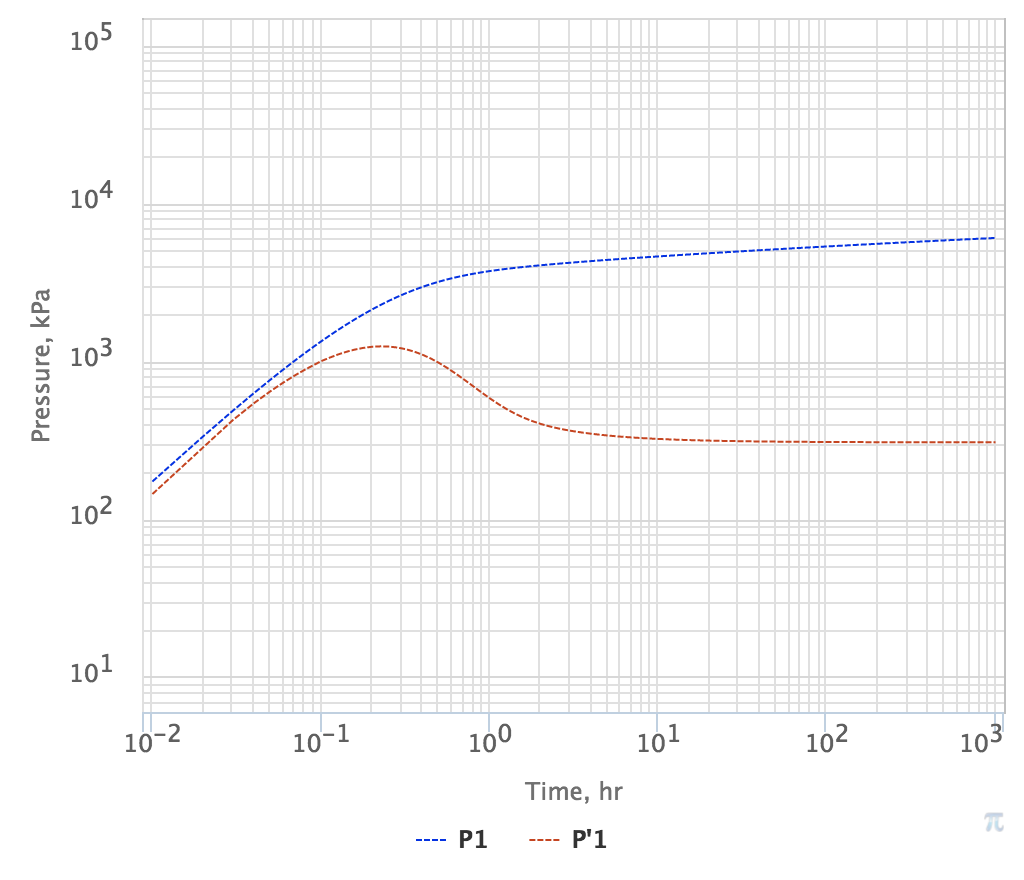
Inputs & Outputs
...
Physical Model
...
Mathematical Model
...
| Expand |
|---|
|
| LaTeX Math Block |
|---|
| r_{wf} < r \leq r_e |
|
| LaTeX Math Block |
|---|
| \frac{\partial p}{\partial t} = \chi \, \left( \frac{\partial^2 p}{\partial r^2} + \frac{1}{r} \frac{\partial p}{\partial r} \right) |
|
| LaTeX Math Block |
|---|
| p(t = 0, {\bf r}) = p_i |
|
| LaTeX Math Block |
|---|
| p(t, r \rightarrow r_e ) = p_i) |
or | LaTeX Math Block |
|---|
| \left[ \frac{\partial p}{\partial r} \right]_{r =r_e} = 0 |
|
| LaTeX Math Block |
|---|
| \left[ r\frac{\partial p(t, r )}{\partial r} \right]_{r \rightarrow r_w} = \frac{q_t}{2 \pi \sigma} |
|
| LaTeX Math Block |
|---|
| p_{wf}(t)= p(t,r_w) - S \cdot r_w \, \frac{\partial p}{\partial r} \Bigg|_{r=r_w} |
|
|
| Expand |
|---|
|
There is no universal analytical solution to the above problem | LaTeX Math Block Reference |
|---|
|
–| LaTeX Math Block Reference |
|---|
|
but it can be always presented as below:
| LaTeX Math Block |
|---|
| p(t,r) = p_i - \frac{q_t}{4 \pi \sigma} \, F \bigg( - \frac{r^2}{4 \chi t} \bigg) |
|
| LaTeX Math Block |
|---|
| p_{wf}(t) = p_i - \frac{q_t}{4 \pi \sigma} \, \bigg[2S + F \bigg( - \frac{r_w^2}{4 \chi t} \bigg) \bigg] |
|
where is a single-argument function describing the peculiarities of the diffusion model (well geometry, penetration geometry, formation inhomogeneities, hydraulic fractures, boundary conditions, etc.).The fact that solution of equations | LaTeX Math Block Reference |
|---|
|
–| LaTeX Math Block Reference |
|---|
|
can be presented as | LaTeX Math Block Reference |
|---|
|
–| LaTeX Math Block Reference |
|---|
|
finds a lot of practical applications in Well Testing.
|
...
| Expand |
|---|
| title | Productivity Index Analysis |
|---|
|
The instantaneous Total Sandface Productivity Index for low-compressibility fluid and low-compressibility rocks does not depend on formation pressure, bottomhole pressure and the flowrate and can be expressed as: | LaTeX Math Block |
|---|
| J_t(t) = \frac{q_t}{p_i - p_{wf}(t)} =\frac{ 2 \pi \sigma }{ S - 0.5 \, F \left( - \frac{r_w^2}{4 \chi t} \right) } |
|
...