Motivation

In many practical cases the reservoir fluid flow created by well is getting aligned with a radial direction towards or away from well.

This type of reservoir fluid flow is called radial fluid flow and corresponding pressure diffusion models provide a diagnostic basis for pressure-rate base reservoir flow analysis.

The radial flow can be infinite acting or boundary dominated or transiting from one to another.

Although the actual reservoir fluid flow may not have an axial symmetry around the well-reservoir contact or around reservoir inhomogeneities (like boundary and faults and composite areas) but still in many practical cases the reservoir flow tends to become radial after some time which makes a Radial Flow Pressure Diffusion @model (in its general form or in particular BVP solution) a popular diagnostic tool.

Inputs & Outputs

Inputs		Outputs
$\begin{array}{l}q_t\end{array}$	total sandface rate	$\begin{array}{l}p(t,r)\end{array}$	reservoir pressure
$\begin{array}{l}{p_i}\end{array}$	initial formation pressure	$\begin{array}{l}{p_{wf}(t)}\end{array}$	well bottomhole pressure
$\begin{array}{l}\sigma\end{array}$	transmissibility, $\begin{array}{l}\sigma = \frac{k \, h}{\mu}\end{array}$
$\begin{array}{l}\chi\end{array}$	pressure diffusivity, $\begin{array}{l}\chi = \frac{k}{\mu} \, \frac{1}{\phi \, c_t}\end{array}$
$\begin{array}{l}S\end{array}$	skin-factor
$\begin{array}{l}r_w\end{array}$	wellbore radius
$\begin{array}{l}r_e\end{array}$	drainage radius (could be infinite)

Detailing

$\begin{array}{l}k\end{array}$	absolute permeability	$\begin{array}{l}c_t\end{array}$	total compressibility, $\begin{array}{l}c_t = c_r + c\end{array}$
$\begin{array}{l}h\end{array}$	effective thickness	$\begin{array}{l}{c_r}\end{array}$	pore compressibility
$\begin{array}{l}\mu\end{array}$	dynamic fluid viscosity	$\begin{array}{l}c\end{array}$	fluid compressibility
$\begin{array}{l}{\phi}\end{array}$	porosity

Physical Model

Radial fluid flow	Homogenous reservoir	Infinite boundary	Zero wellbore radius	Slightly compressible fluid flow	Constant rate	Constant skin
$\begin{array}{l}p(t, {\bf r}) \rightarrow p(t, r)\end{array}$ $\begin{array}{l}{\bf r} \in ℝ^2 = \{ x, y\}\end{array}$	$\begin{array}{l}M(r, p)=M =\rm const\end{array}$ $\begin{array}{l}\phi(r, p)=\phi =\rm const\end{array}$ $\begin{array}{l}h(r)=h =\rm const\end{array}$ $\begin{array}{l}c_r(r)=c_r =\rm const\end{array}$	$\begin{array}{l}r \rightarrow \infty\end{array}$	$\begin{array}{l}r_w = 0\end{array}$	$\begin{array}{l}c_t(r,p) = \rm const\end{array}$	$\begin{array}{l}q_t = \rm const\end{array}$	$\begin{array}{l}S = \rm const\end{array}$

Mathematical Model

Definition

(1)	$\begin{array}{l}\displaystyle r_{wf} < r \leq r_e\end{array}$

(2)	$\begin{array}{l}\displaystyle \frac{\partial p}{\partial t} = \chi \, \left( \frac{\partial^2 p}{\partial r^2} + \frac{1}{r} \frac{\partial p}{\partial r} \right)\end{array}$

(3)	$\begin{array}{l}\displaystyle p(t = 0, {\bf r}) = p_i\end{array}$

(4)	$\begin{array}{l}\displaystyle p(t, r \rightarrow r_e ) = p_i)\end{array}$

or

(5)	$\begin{array}{l}\displaystyle \left[ \frac{\partial p}{\partial r} \right]_{r =r_e} = 0\end{array}$

(6)	$\begin{array}{l}\displaystyle \left[ r\frac{\partial p(t, r )}{\partial r} \right]_{r \rightarrow r_w} = \frac{q_t}{2 \pi \sigma}\end{array}$

(7)	$\begin{array}{l}\displaystyle p_{wf}(t)= p(t,r_w) - S \cdot r_w \, \frac{\partial p}{\partial r} \Bigg\|_{r=r_w}\end{array}$

Solution

There is no universal analytical solution to the above problem (1)– (7) but it can be always presented as below:

(8)	$\begin{array}{l}\displaystyle p(t,r) = p_i - \frac{q_t}{4 \pi \sigma} \, F \bigg( - \frac{r^2}{4 \chi t} \bigg)\end{array}$

(9)	$\begin{array}{l}\displaystyle p_{wf}(t) = p_i - \frac{q_t}{4 \pi \sigma} \, \bigg[2S + F \bigg( - \frac{r_w^2}{4 \chi t} \bigg) \bigg]\end{array}$

where $\begin{array}{l}F(\xi)\end{array}$ is a single-argument function describing the peculiarities of the diffusion model (well geometry, penetration geometry, formation inhomogeneities, hydraulic fractures, boundary conditions, etc.).

The fact that solution of equations (1)– (7) can be presented as (8)– (9) finds a lot of practical applications in Well Testing.

Derivation

Applications

Equations (8) and (9) show how the basic diffusion model parameters impact the pressure response while other diffusion parameters are encoded in $\begin{array}{l}F\end{array}$ function and play important methodological role as they are used in many algorithms and express-methods of Pressure Testing.

Line Source Solution

In case of infinite homogeneous reservoir, produced by a infinitely small vertical well with no skin and no wellbore storage the $\begin{array}{l}F\end{array}$ function has an exact analytical formula, given by exponential integral $\begin{array}{l}F(z) = - {\rm Ei} (z)\end{array}$ (see Line Source Solution (LSS) @model).

PTA

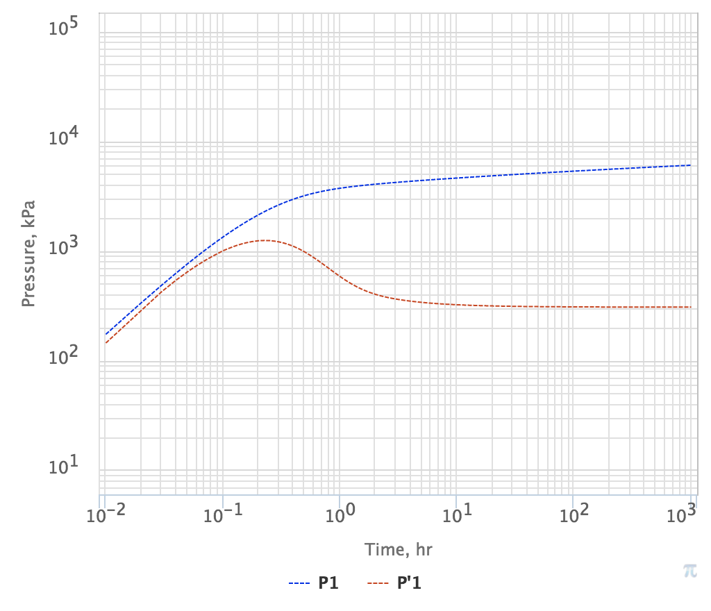
PTA – Pressure Transient Analysis

Pressure Drop

(10)	$\begin{array}{l}\displaystyle \delta p = p_i - p_{wf}(t) \sim \ln t + {\rm const}\end{array}$

Log derivative

(11)	$\begin{array}{l}\displaystyle t \frac{d (\delta p)}{dt} \sim \rm const\end{array}$

Fig. 2. PTA Diagnostic plot for radial fluid flow

Productivity Index Analysis

The instantaneous Total Sandface Productivity Index for low-compressibility fluid and low-compressibility rocks does not depend on formation pressure, bottomhole pressure and the flowrate and can be expressed as:

(12)	$\begin{array}{l}\displaystyle J_t(t) = \frac{q_t}{p_i - p_{wf}(t)} =\frac{ 2 \pi \sigma }{ S - 0.5 \, F \left( - \frac{r_w^2}{4 \chi t} \right) }\end{array}$

Isobar Propagation

Isobar equation for a constant-rate production:

(13)	$\begin{array}{l}\displaystyle p(t,r) = p_i + \frac{q_t}{4 \pi \sigma} \, F \bigg( - \frac{r^2}{4 \chi t} \bigg) = {\rm const} \quad \rightarrow \quad \frac{r^2}{4 \chi t}= {\rm const}\end{array}$

Since the pressure disturbance at $\begin{array}{l}t=0\end{array}$ moment was at well walls $\begin{array}{l}r=r_w\end{array}$ then the formula for constant-pressure front propagation becomes:

(14)	$\begin{array}{l}\displaystyle r(t) = r_w + 2 \sqrt{\chi t}\end{array}$

This leads to estimation of isobar velocity:

(15)	$\begin{array}{l}\displaystyle u_p(t) = \sqrt{\frac{\chi}{t}}\end{array}$

Page tree

Motivation

Inputs & Outputs

Physical Model

Mathematical Model

Applications

See Also