Motivation
...
In many practical cases the reservoir flow created by a well or group of wells is getting aligned with a specific linear direction away from wellwells (see linear fluid flow).
This happens when well is wells are placed in a channel or a narrow compartment.
It also happens around fracture planes and conductive faults. It also develops temporarily at early times of the transients in horizontal wells.
This type of flow is called linear fluid flow and a corresponding PTA type library model models provides a reference for linear fluid flow diagnostics.
Inputs & Outputs
...
...
...
| sigma = \frac{k \, h}{\mu} |
|
|
...
| LaTeX Math Inline |
|---|
| body | \chi = \frac{k}{\mu} \, \frac{1}{\phi \, c_t} |
|---|
|
|
|
|
Physical Model
...
...
Physical Model
...
mathinline| body | p(t, x)Homogeneous reservoir | c_t(, p) = c_r +c = \rm const | | p(t, {\bf r}) \rightarrow p(t, x) |
|
| LaTeX Math Inline |
|---|
| body | {\bf r} \in ℝ^2 = \{ x, y\} |
|---|
|
|
| LaTeX Math Inline |
|---|
| body | \phi(x, p)=\phi =\rm const |
|---|
|
|
Infinite boundary | | LaTeX Math Inline |
|---|
| body | 0 \leq x \rightarrow \infty |
|---|
|
| | | LaTeX Math Inline |
|---|
| body | c_t(p) = c_r +c = \rm const |
|---|
|
| |
Mathematical Model
...
| Expand |
|---|
|
| LaTeX Math Block |
|---|
| \frac{\partial p}{\partial t} = \chi \, \frac{d^2 p}{dx^2} |
|
| LaTeX Math Block |
|---|
| p(t = 0, x) = p_i |
|
| LaTeX Math Block |
|---|
| p(t, x \rightarrow \infty ) = p_i |
|
| LaTeX Math Block |
|---|
| \frac{\partial p(t, x )}{\partial x} \bigg|_{x \rightarrow 0} = \frac{q_t}{\sigma \, d} |
|
|
| Expand |
|---|
|
| LaTeX Math Block |
|---|
| p(t,x) = p_i - \frac{q_t}{\sigma \, d} \bigg[ \sqrt{\frac{4 \chi t}{\pi}} \exp \bigg( -\frac{x^2}{4 \chi t} \bigg) - x \, \bigg[ 1- {\rm erf} \bigg(\frac{x}{\sqrt{4 \, \chi \, t}} \bigg) \bigg] \bigg] |
|
| LaTeX Math Block |
|---|
| p_{wf}(t) = p(t,x=0)= p_i - \frac{q_t}{\sigma \, d} \, \sqrt{\frac{4 \chi t}{\pi}} |
|
|
...
Applications
...
...
...
...
See also
...
Physics / Fluid Dynamics / Linear fluid flow
[ Radial Flow Pressure @model ] [ 1DR pressure diffusion of low-compressibility fluid ] [ Exponential Integral ]
[ Petroleum Industry / Upstream / Subsurface E&P Disciplines / Well Testing / Pressure Testing ]
| Show If |
|---|
|
| Panel |
|---|
|
| Expand |
|---|
| 1 1DL low-compressibility diffusion in infinite homogeneous reservoir
Рассмотрим плоскопараллельный однородный пласт постоянной толщины ограниченный в горизонтальной плоскости полосой ширины с координатой вдоль полосы, которая вскрыта горизонтальной скважиной в точке по всей ширине полосы (например, компартмент между двумя параллельными непроницаемыми разломами) и начальным пластовым давлением .
Пусть в момент времени скважина запускается с дебитом (в пластовых условиях).Диффузия давления описывается решением уравнения однофазного линейного течения в бесконечном однородном пласте | LaTeX Math Block |
|---|
| \frac{\partial p}{\partial t} = \chi \, \frac{d^2 p}{dx^2} |
с начальным условием | LaTeX Math Block |
|---|
| p(t = 0, x) = p_i |
и граничными условиями | LaTeX Math Block |
|---|
| p(t, x \rightarrow \infty ) = p_i |
| LaTeX Math Block |
|---|
| \frac{\partial p(t, x )}{\partial x} \bigg|_{x \rightarrow 0} = \frac{q_t}{\sigma \, d} |
где | LaTeX Math Inline |
|---|
| body | \sigma = \frac{k \, h}{\mu} |
|---|
|
– гидропроводность пласта, | LaTeX Math Inline |
|---|
| body | \chi = \frac{k}{\mu} \, \frac{1}{\phi \, c_t} |
|---|
|
– пьезопроводность пласта, – проницаемость пласта, – пористость пласта, – сжимаемость пласта, – сжимаемость порового объема трещины, – сжимаемость флюида, насыщающего пласт, – вязкость флюида, насыщающего пласт.
Решение этого уравнения дается следующим выражением:
| LaTeX Math Block |
|---|
| p(t,x) = p_i - \frac{q_t}{\sigma \, d} \bigg[ \sqrt{\frac{4 \chi t}{\pi}} \exp \bigg( -\frac{x^2}{4 \chi t} \bigg) - x \, \bigg[ 1- {\rm erf} \bigg(\frac{x}{\sqrt{4 \, \chi \, t}} \bigg) \bigg] \bigg] |
В стволе скважины ( ) динамика давления будет описываться следующей формулой:| LaTeX Math Block |
|---|
| p_{wf}(t) = p_i - \frac{q_t}{\sigma \, d} \, \sqrt{\frac{4 \chi t}{\pi}} |
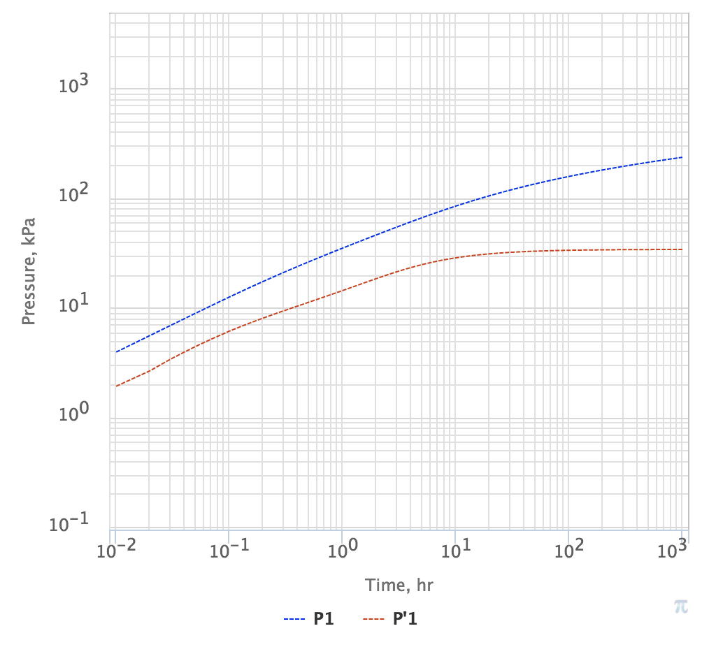
Отсюда следует что динамическая депрессия на пласт растет пропорционально квадратному корню из времени | LaTeX Math Block |
|---|
| \delta p = p_i - p_{wf}(t) \sim t^{1/2} |
равно как и ее логарифмическая производная | LaTeX Math Block |
|---|
| t \frac{d (\delta p)}{dt} \sim t^{1/2} |
В лог-лог координатах депрессия и ее лог-производная будут иметь одинаковый слоп 1/2, что является характерным для линейно-одномерной фильтрации.
q |
|
|
...