...
Although the actual reservoir fluid flow may not have an axial symmetry around the well-reservoir contact or around reservoir inhomogeneities (like boundary and faults and composite areas) but still in still in many practical cases the long-term correlation between the flowrate and bottom-hole pressure response can be approximated by a radial flow pressure modelthe reservoir flow tends to become radial after some time which makes a Radial Flow Pressure Diffusion @model (in its general form or in particular BVP solution) a popular diagnostic tool.
Inputs & Outputs
...
Physical Model
...
Mathematical Model
...
| Expand |
|---|
|
| LaTeX Math Block |
|---|
| r_{wf} < r \leq r_e |
|
| LaTeX Math Block |
|---|
| \frac{\partial p}{\partial t} = \chi \, \left( \frac{\partial^2 p}{\partial r^2} + \frac{1}{r} \frac{\partial p}{\partial r} \right) |
|
| LaTeX Math Block |
|---|
| p(t = 0, {\bf r}) = p_i |
|
| LaTeX Math Block |
|---|
| p(t, r \rightarrow r_e ) = p_i) |
or | LaTeX Math Block |
|---|
| \left[ \frac{\partial p}{\partial r} \right]_{r =r_e} = 0 |
|
| LaTeX Math Block |
|---|
| \left[ r\frac{\partial p(t, r )}{\partial r} \right]_{r \rightarrow r_w} = \frac{q_t}{2 \pi \sigma} |
|
| LaTeX Math Block |
|---|
| p_{wf}(t)= p(t,r_w) - S \cdot r_w \, \frac{\partial p}{\partial r} \Bigg|_{r=r_w} |
|
|
| Expand |
|---|
|
There is no universal analytical solution to the above problem | LaTeX Math Block Reference |
|---|
|
–| LaTeX Math Block Reference |
|---|
|
but it can be always presented as below:
| LaTeX Math Block |
|---|
| p(t,r) = p_i - \frac{q_t}{4 \pi \sigma} \, F \bigg( - \frac{r^2}{4 \chi t} \bigg) |
|
| LaTeX Math Block |
|---|
| p_{wf}(t) = p_i - \frac{q_t}{4 \pi \sigma} \, \bigg[2S + F \bigg( - \frac{r_w^2}{4 \chi t} \bigg) \bigg] |
|
where is a single-argument function describing the peculiarities of the diffusion model (well geometry, penetration geometry, formation inhomogeneities, hydraulic fractures, boundary conditions, etc.).The fact that solution of equations | LaTeX Math Block Reference |
|---|
|
–| LaTeX Math Block Reference |
|---|
|
can be presented as | LaTeX Math Block Reference |
|---|
|
–| LaTeX Math Block Reference |
|---|
|
finds a lot of practical applications in Well Testing.
|
...
Equations
| LaTeX Math Block Reference |
|---|
|
and
| LaTeX Math Block Reference |
|---|
|
show how the
basic diffusion model parameters impact the pressure response while other diffusion parameters are encoded in
function and play important methodological role as they are used in many algorithms and express-methods of
Pressure Testing.In many practical cases the reservoir flow tends to become radial after some time which makes a radial flow pressure diffusion a popular diagnostic tool.
| Expand |
|---|
| title | Line Source Solution |
|---|
|
In case of infinite homogeneous reservoir, produced by a infinitely small vertical well with no skin and no wellbore storage the function has an exact analytical formula, given by exponential integral | LaTeX Math Inline |
|---|
| body | F(z) = - {\rm Ei} (z) |
|---|
|
(see Line Source Solution (LSS) @model).
|
...
| Expand |
|---|
| title | Productivity Index Analysis |
|---|
|
The instantaneous Total Sandface Productivity Index for low-compressibility fluid and low-compressibility rocks does not depend on formation pressure, bottomhole pressure and the flowrate and can be expressed as: | LaTeX Math Block |
|---|
| J_t(t) = \frac{q_t}{p_i - p_{wf}(t)} =\frac{ 2 \pi \sigma }{ S - 0.5 \, F \left( - \frac{r_w^2}{4 \chi t} \right) } |
|
...
Physics / Mechanics / Continuum mechanics / Fluid Mechanics / Fluid Dynamics / Radial fluid flow / Pressure diffusion / Pressure Diffusion @model
Petroleum Industry / Upstream / Subsurface E&P Disciplines / Well Testing / Pressure Testing
[ Well & Reservoir Surveillance ]
[ Pressure diffusion @model ][ Line Source Solution (LSS) @model ] [ Linear Flow Pressure Diffusion @model ]
| Show If |
|---|
|
| Panel |
|---|
|
| Expand |
|---|
| but this only works for the middle-times and long-times as early times are influenced by wellbore storage and non-linear effects of skin.
| Expand |
|---|
| | Include Page |
|---|
| Line Source Solution (LSS) |
|---|
| Line Source Solution (LSS) |
|---|
|
|
| LaTeX Math Block |
|---|
| p(t,r) = p_i + \frac{q_t}{4 \pi \sigma} \, {\rm Ei} \bigg( - \frac{r^2}{4 \chi t} \bigg) |
Рассмотрим плоскопараллельный аксиально-симметричный однородный пласт постоянной толщины , с радиальной координатой в перпендикулярной к оси скважины плоскости, который вскрыт бесконечно тонкой скважиной в точке (где – радиальная координата в перпендикулярной к оси скважине плоскости) и начальным пластовым давлением .
Пусть в момент времени
скважина запускается с дебитом (в пересчете на пластовые условия).Диффузия давления описывается решением уравнения однофазного радиального течения в бесконечном однородном пласте: | LaTeX Math Block |
|---|
| \frac{\partial p}{\partial t} = \chi \, \Delta p = \chi \, \frac{1}{r} \frac{\partial}{\partial r} \bigg( r \frac{\partial p}{\partial r} \bigg) |
с начальным условием: | LaTeX Math Block |
|---|
| p(t = 0, r) = p_i |
и граничными условиями: | LaTeX Math Block |
|---|
| p(t, r \rightarrow \infty ) = p_i |
| LaTeX Math Block |
|---|
| anchor | Boundary_q |
|---|
| alignment | left |
|---|
| r \frac{\partial p(t, x )}{\partial r} \bigg|_{r \rightarrow 0} = \frac{q_t}{2 \pi \sigma} |
где | LaTeX Math Inline |
|---|
| body | \sigma = \frac{k \, h}{\mu} |
|---|
|
– гидропроводность пласта, | LaTeX Math Inline |
|---|
| body | \chi = \frac{k}{\mu} \, \frac{1}{\phi \, c_t} |
|---|
|
– пьезопроводность пласта, – проницаемость пласта, – пористость пласта, – сжимаемость пласта, – сжимаемость порового коллектора, – сжимаемость насыщающего пласт флюида, – вязкость насыщающего пласт флюида.
При анализе отклика давления на самой скважине ( ) после включения на достаточно больших временах, удовлетворяющих условию:| LaTeX Math Block |
|---|
| t \gg \frac{r_w^2}{4 \chi}
|
которые на практике наступают очень быстро, можно воспользоваться приближением | LaTeX Math Inline |
|---|
| body | {\rm Ei}(-x) \sim \ln (x) + \gamma \sim \ln (1.781 x) |
|---|
|
, где – постоянная Эйлера.
Режим радиального течения к линейному источнику примет вид:
| LaTeX Math Block |
|---|
| p(t,r_w) = p_i + \frac{q_t}{4 \pi \sigma} \, \ln \bigg( 1.781 \, \frac{r_w^2}{4 \chi t} \bigg) |
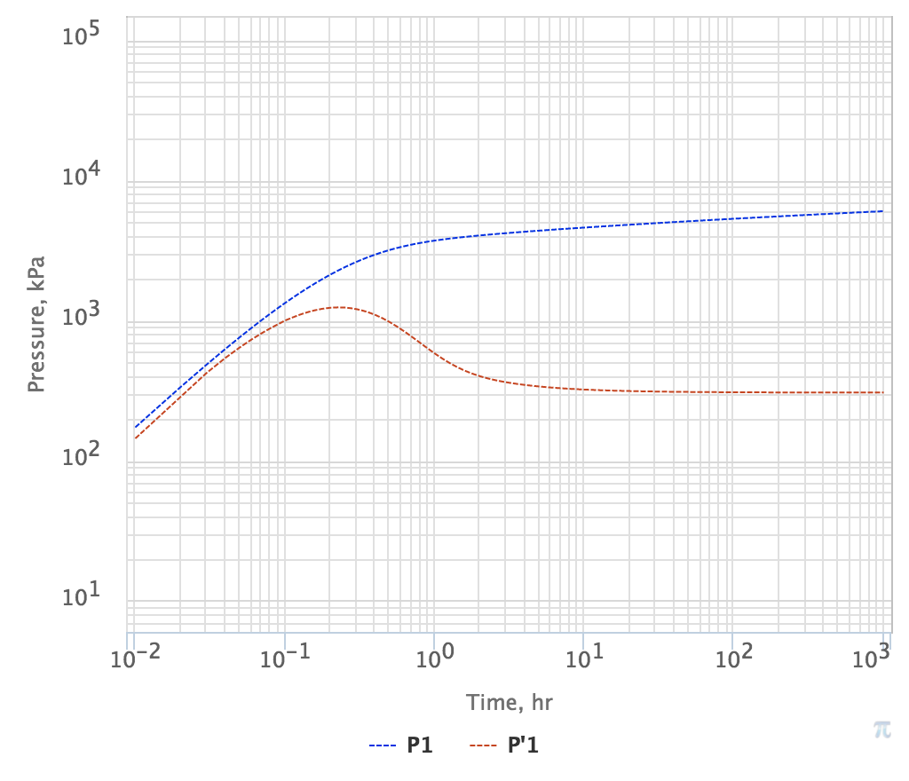
Отсюда следует, что уже вскоре после запуска скважины динамическая депрессия на пласт начинает логарифмически расти во времени:
| LaTeX Math Block |
|---|
| \delta p = p_i - p_{wf}(t) \sim { \rm const } + \frac{q_t}{4 \pi \sigma} \, \ln t |
а логарифмическая производная становится постоянной во времени: | LaTeX Math Block |
|---|
| t \frac{d (\delta p)}{dt} \sim \frac{q_t}{4 \pi \sigma} |
В лог-лог координатах лог-производная депрессии будет горизонтальной, что является характерным для радиальной фильтрации в бесконечном пласте.
|
|
|
...