...
This type of flow is called linear fluid flow and corresponding PTA type library models provides a reference for linear fluid flow diagnostics.
Inputs & Outputs
...
Physical Model
...
Mathematical Model
...
| Expand |
|---|
|
| LaTeX Math Block |
|---|
| \frac{\partial p}{\partial t} = \chi \, \frac{d^2 p}{dx^2} |
|
| LaTeX Math Block |
|---|
| p(t = 0, x) = p_i |
|
| LaTeX Math Block |
|---|
| p(t, x \rightarrow \infty ) = p_i |
|
| LaTeX Math Block |
|---|
| \frac{\partial p(t, x )}{\partial x} \bigg|_{x \rightarrow 0} = \frac{q_t}{\sigma \, d} |
|
|
| Expand |
|---|
|
| LaTeX Math Block |
|---|
| p(t,x) = p_i - \frac{q_t}{\sigma \, d} \bigg[ \sqrt{\frac{4 \chi t}{\pi}} \exp \bigg( -\frac{x^2}{4 \chi t} \bigg) - x \, \bigg[ 1- {\rm erf} \bigg(\frac{x}{\sqrt{4 \, \chi \, t}} \bigg) \bigg] \bigg] |
|
| LaTeX Math Block |
|---|
| p_{wf}(t) = p(t,x=0)= p_i - \frac{q_t}{\sigma \, d} \, \sqrt{\frac{4 \chi t}{\pi}} |
|
|
Applications
...
See also
...
Physics / Fluid Dynamics / Linear fluid flow
[ Radial Flow Pressure Diffusion @model@model ] [ 1DR pressure diffusion of low-compressibility fluid ] [ Exponential Integral ]
[ Petroleum Industry / Upstream / Subsurface E&P Disciplines / Well Testing / Pressure Testing ]
| Show If |
|---|
|
| Panel |
|---|
|
| Expand |
|---|
| 1 1DL low-compressibility diffusion in infinite homogeneous reservoir
Рассмотрим плоскопараллельный однородный пласт постоянной толщины ограниченный в горизонтальной плоскости полосой ширины с координатой вдоль полосы, которая вскрыта горизонтальной скважиной в точке по всей ширине полосы (например, компартмент между двумя параллельными непроницаемыми разломами) и начальным пластовым давлением .
Пусть в момент времени скважина запускается с дебитом (в пластовых условиях).Диффузия давления описывается решением уравнения однофазного линейного течения в бесконечном однородном пласте | LaTeX Math Block |
|---|
| \frac{\partial p}{\partial t} = \chi \, \frac{d^2 p}{dx^2} |
с начальным условием | LaTeX Math Block |
|---|
| p(t = 0, x) = p_i |
и граничными условиями | LaTeX Math Block |
|---|
| p(t, x \rightarrow \infty ) = p_i |
| LaTeX Math Block |
|---|
| \frac{\partial p(t, x )}{\partial x} \bigg|_{x \rightarrow 0} = \frac{q_t}{\sigma \, d} |
где | LaTeX Math Inline |
|---|
| body | \sigma = \frac{k \, h}{\mu} |
|---|
|
– гидропроводность пласта, | LaTeX Math Inline |
|---|
| body | \chi = \frac{k}{\mu} \, \frac{1}{\phi \, c_t} |
|---|
|
– пьезопроводность пласта, – проницаемость пласта, – пористость пласта, – сжимаемость пласта, – сжимаемость порового объема трещины, – сжимаемость флюида, насыщающего пласт, – вязкость флюида, насыщающего пласт.
Решение этого уравнения дается следующим выражением:
| LaTeX Math Block |
|---|
| p(t,x) = p_i - \frac{q_t}{\sigma \, d} \bigg[ \sqrt{\frac{4 \chi t}{\pi}} \exp \bigg( -\frac{x^2}{4 \chi t} \bigg) - x \, \bigg[ 1- {\rm erf} \bigg(\frac{x}{\sqrt{4 \, \chi \, t}} \bigg) \bigg] \bigg] |
В стволе скважины ( ) динамика давления будет описываться следующей формулой:| LaTeX Math Block |
|---|
| p_{wf}(t) = p_i - \frac{q_t}{\sigma \, d} \, \sqrt{\frac{4 \chi t}{\pi}} |
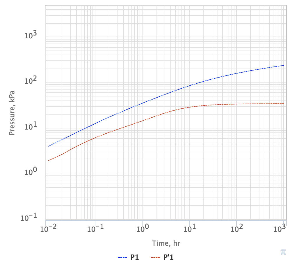
Отсюда следует что динамическая депрессия на пласт растет пропорционально квадратному корню из времени | LaTeX Math Block |
|---|
| \delta p = p_i - p_{wf}(t) \sim t^{1/2} |
равно как и ее логарифмическая производная | LaTeX Math Block |
|---|
| t \frac{d (\delta p)}{dt} \sim t^{1/2} |
В лог-лог координатах депрессия и ее лог-производная будут иметь одинаковый слоп 1/2, что является характерным для линейно-одномерной фильтрации.
q |
|
|
...