Motivation

In many practical cases the reservoir flow created by well is getting aligned with a radial direction towards or away from well.

This type of flow is called radial fluid flow and corresponding pressure diffusion models provide a diagnostic basis for pressure-rate base reservoir flow analysis.

Although the actual flow may not have an axial symmetry around the well-reservoir contact or reservoir inhomogeneities (like boundary and faults and composite areas) but still:

the dominant part of wellbore and reservoir pressure variation is usually radial-flow or linear-flow and the two represent the basis for Pressure diffusion analysis
in most practical cases the long-term correlation between the flowrate and bottom-hole pressure response can be approximated by a radial flow pressure model

Inputs & Outputs

Inputs		Outputs
$\begin{array}{l}q_t\end{array}$	total sandface rate	$\begin{array}{l}p(t,r)\end{array}$	reservoir pressure
$\begin{array}{l}{p_i}\end{array}$	initial formation pressure	$\begin{array}{l}{p_{wf}(t)}\end{array}$	well bottomhole pressure
$\begin{array}{l}\sigma\end{array}$	transmissibility
$\begin{array}{l}\chi\end{array}$	pressure diffusivity

Detailing

$\begin{array}{l}\sigma = \frac{k \, h}{\mu}\end{array}$	transmissibility	$\begin{array}{l}\mu\end{array}$	dynamic fluid viscosity
$\begin{array}{l}\chi = \frac{k}{\mu} \, \frac{1}{\phi \, c_t}\end{array}$	pressure diffusivity	$\begin{array}{l}c_t = c_r + c\end{array}$	total compressibility
$\begin{array}{l}k\end{array}$	absolute permeability	$\begin{array}{l}{c_r}\end{array}$	pore compressibility
$\begin{array}{l}{\phi}\end{array}$	porosity	$\begin{array}{l}c\end{array}$	fluid compressibility

Physical Model

Radial fluid flow	Homogenous reservoir	Infinite boundary	Zero wellbore radius	Slightly compressible fluid flow	Constant rate	Constant Skin
$\begin{array}{l}p(t, r)\end{array}$	$\begin{array}{l}M(r, p)=M =\rm const\end{array}$ $\begin{array}{l}\phi(r, p)=\phi =\rm const\end{array}$ $\begin{array}{l}h(r)=h =\rm const\end{array}$ $\begin{array}{l}c_r(r)=c_r =\rm const\end{array}$	$\begin{array}{l}r \rightarrow \infty\end{array}$	$\begin{array}{l}r_w = 0\end{array}$	$\begin{array}{l}c_t(r,p) = \rm const\end{array}$	$\begin{array}{l}q_t = \rm const\end{array}$	$\begin{array}{l}S = \rm const\end{array}$

Mathematical Model

Definition

(1)	$\begin{array}{l}\displaystyle \frac{\partial p}{\partial t} = \chi \, \left( \frac{\partial^2 p}{\partial r^2} + \frac{1}{r} \frac{\partial p}{\partial r} \right)\end{array}$

(2)	$\begin{array}{l}\displaystyle p(t = 0, {\bf r}) = p_i\end{array}$

(3)	$\begin{array}{l}\displaystyle p(t, r \rightarrow \infty ) = p_i\end{array}$

(4)	$\begin{array}{l}\displaystyle \left[ r\frac{\partial p(t, r )}{\partial r} \right]_{r \rightarrow r_w} = \frac{q_t}{2 \pi \sigma}\end{array}$

Solution

(5)	$\begin{array}{l}\displaystyle p(t,r) = p_i + \frac{q_t}{4 \pi \sigma} \, F \bigg( - \frac{r^2}{4 \chi t} \bigg)\end{array}$

(6)	$\begin{array}{l}\displaystyle p_{wf}(t) = p_i + \frac{q_t}{4 \pi \sigma} \, \bigg[ - 2S + F \bigg( - \frac{r_w^2}{4 \chi t} \bigg) \bigg]\end{array}$

where $\begin{array}{l}F(\xi)\end{array}$ a single-argument function describing the peculiarities of the diffusion model (well geometry, penetration geometry, formation inhomogeneities, hydraulic fractures, boundary conditions, etc.)

Derivation

Applications

Line Source Solution

In simplest case of infinite homogeneous reservoir, produced by a vertical well the $\begin{array}{l}F\end{array}$ function has an exact analytical formula, given by exponential integral $\begin{array}{l}F(z) = {\rm Ei}_1 (z)\end{array}$ (see Line Source Solution (LSS) @model).

PTA

Pressure Testing – Infinite reservoir

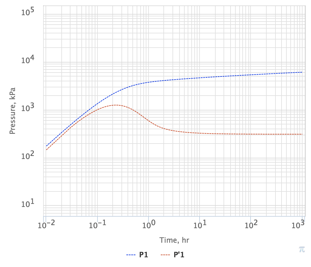
Pressure Drop

(7)	$\begin{array}{l}\displaystyle \delta p = p_i - p_{wf}(t) \sim \ln t + {\rm const}\end{array}$

Log derivative

(8)	$\begin{array}{l}\displaystyle t \frac{d (\delta p)}{dt} \sim \rm const\end{array}$

Fig. 2. PTA Diagnostic plot for radial fluid flow

Productivity Index Analysis

The Productivity Index for single-phase low-compressibility fluid and low-compressibility rocks does not depend on formation pressure, bottom-hole pressure and the flow rate and can be expressed as:

(9)	$\begin{array}{l}\displaystyle J(t) = \frac{q_t}{p_i - p_{wf}(t)} =\frac{ 4 \pi \sigma }{ 2S - F \bigg( - \frac{r_w^2}{4 \chi t} \bigg) }\end{array}$

Isobar Propagation

Isobar equation for a constant-rate production:

(10)	$\begin{array}{l}\displaystyle p(t,r) = p_i + \frac{q_t}{4 \pi \sigma} \, F \bigg( - \frac{r^2}{4 \chi t} \bigg) = {\rm const} \quad \rightarrow \quad \frac{r^2}{4 \chi t}= {\rm const}\end{array}$

Since the pressure disturbance at $\begin{array}{l}t=0\end{array}$ moment was at well walls $\begin{array}{l}r=r_w\end{array}$ then the formula for constant-pressure front propagation becomes:

(11)	$\begin{array}{l}\displaystyle r(t) = r_w + 2 \sqrt{\chi t}\end{array}$

This leads to estimation of isobar velocity:

(12)	$\begin{array}{l}\displaystyle u_p(t) = \sqrt{\frac{\chi}{t}}\end{array}$

Page tree

Motivation

Inputs & Outputs

Physical Model

Mathematical Model

Applications

See also

Page tree

Radial Flow Pressure Diffusion @model

Motivation

Inputs & Outputs

Physical Model

Mathematical Model

Applications

See also