Motivation

Reservoir pressure dynamics away from wellbore and boundaries is representative of two very important complex reservoir properties: transmissibility $\begin{array}{l}\sigma\end{array}$ and pressure diffusivity $\begin{array}{l}\chi\end{array}$ .

In case the reservoir flow has been created by a well (vertical or horizontal) it will trend to form a radial flow away from boundaries and well itself.

In this case a pressure drop and well flowrate can be roughly related to each other by means of a simple analytical homogeneous reservoir flow model with wellbore and boundary effects neglected.

Since the well radius is neglected the well is modeled as a vertical 0-thickness line sourcing the fluid from a reservoir, giving a model a specific name Line Source Solution.

Inputs & Outputs

Inputs		Outputs
$\begin{array}{l}q_t\end{array}$	total sandface rate	$\begin{array}{l}p(t,r)\end{array}$	reservoir pressure
$\begin{array}{l}{p_i}\end{array}$	initial formation pressure
$\begin{array}{l}\sigma\end{array}$	transmissibility
$\begin{array}{l}\chi\end{array}$	pressure diffusivity

Detailing

$\begin{array}{l}\sigma = \frac{k \, h}{\mu}\end{array}$	transmissibility	$\begin{array}{l}\mu\end{array}$	dynamic fluid viscosity
$\begin{array}{l}\chi = \frac{k}{\mu} \, \frac{1}{\phi \, c_t}\end{array}$	pressure diffusivity	$\begin{array}{l}{t}\end{array}$	time
$\begin{array}{l}k\end{array}$	absolute permeability	$\begin{array}{l}{r}\end{array}$	radial direction
$\begin{array}{l}{\phi}\end{array}$	porosity	$\begin{array}{l}{c_t}\end{array}$	total compressibility

Physical Model

Radial fluid flow	Homogenous reservoir	Infinite boundary	Zero wellbore radius	Slightly compressible fluid flow	Constant rate production
$\begin{array}{l}p(t, r)\end{array}$	$\begin{array}{l}M(r, p)=M =\rm const\end{array}$ $\begin{array}{l}\phi(r, p)=\phi =\rm const\end{array}$ $\begin{array}{l}h(r)=h =\rm const\end{array}$ $\begin{array}{l}c_r(r)=c_r =\rm const\end{array}$	$\begin{array}{l}r \rightarrow \infty\end{array}$	$\begin{array}{l}r_w = 0\end{array}$	$\begin{array}{l}c_t(p) = c_r +c = \rm const\end{array}$	$\begin{array}{l}q_t = \rm const\end{array}$

Mathematical Model

Motion equation

Initial condition

Boundary conditions

(1)	$\begin{array}{l}\displaystyle \frac{\partial p}{\partial t} = \chi \, \left[ \frac{\partial^2 p}{\partial t^2} + \frac{1}{r} \frac{\partial p}{\partial r} \right]\end{array}$

(2)	$\begin{array}{l}\displaystyle p(t=0,r) = p_i\end{array}$

(3)	$\begin{array}{l}\displaystyle p(t, r=\infty) = p_i\end{array}$

(4)	$\begin{array}{l}\displaystyle \left[ r \frac{\partial p}{\partial r} \right]_{r=0} = \frac{q_t}{2 \pi \sigma}\end{array}$

Computational Model

(5)	$\begin{array}{l}\displaystyle p(t,r) = p_i + \frac{q_t}{4 \pi \sigma} {\rm Ei} \left(-\frac{r^2}{4 \chi t} \right)\end{array}$

Approximations

Late-time response

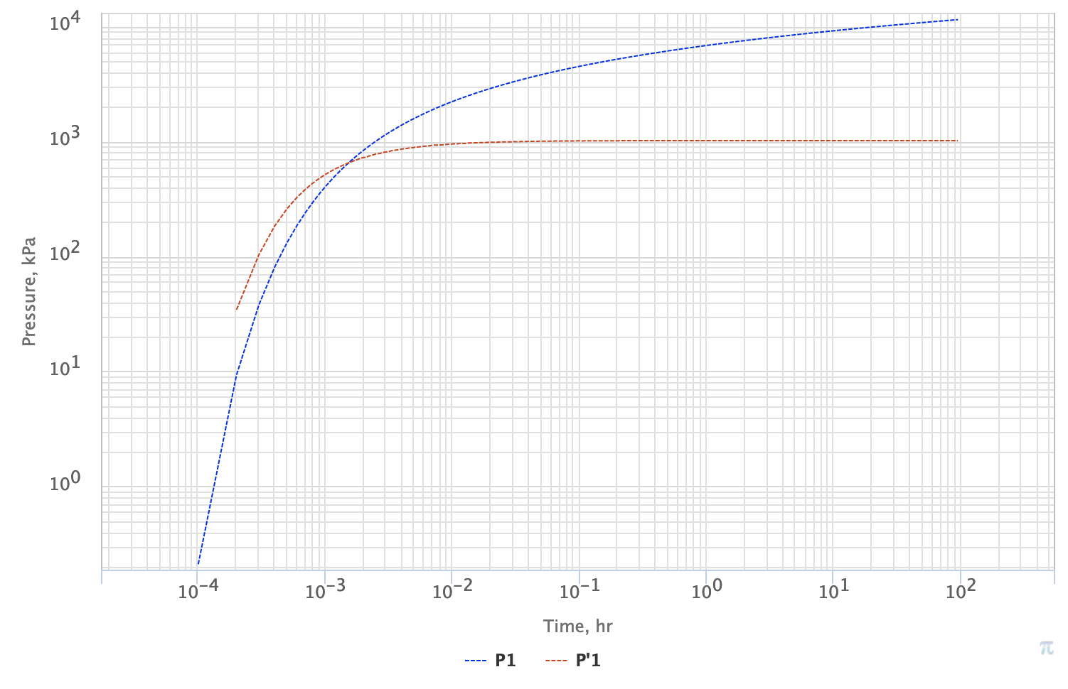
(6)	$\begin{array}{l}\displaystyle p(t,r) \sim p_i + \frac{q_t}{4 \pi \sigma} \left[ \gamma + \ln \left(\frac{r^2}{4 \chi t} \right) \right] = p_i - \frac{q_t}{4 \pi \sigma} \ln \left(\frac{2.24585 \, t}{r^2} \right)\end{array}$

Diagnostic Plots

Pressure Drop

(7)	$\begin{array}{l}\displaystyle \delta p = p_i - p_{wf}(t) = \frac{q_t}{4 \pi \sigma} {\rm Ei} \left(-\frac{r^2}{4 \chi t} \right) \sim \ln t + {\rm const}\end{array}$

Log derivative

(8)	$\begin{array}{l}\displaystyle t \frac{d (\delta p)}{dt} \sim \rm const\end{array}$

Fig. 1. PTA Diagnostic Plot for LSS pressure response for the 0.1 md reservoir in a close line source vicinity (0.1 m), which is about a typical wellbore size.

One can easily see that with wellbore effects neglected even for a very low permeability reservoir the IARF regime is getting formed very early at 0.01 hr (36 s).

Page tree

Motivation

Inputs & Outputs

Physical Model

Mathematical Model

Computational Model

Approximations

Diagnostic Plots

See also

Page tree

Line Source Solution (LSS) @model

Motivation

Inputs & Outputs

Physical Model

Mathematical Model

Computational Model

Approximations

Diagnostic Plots

See also