Motivation

The most accurate way to simulate Aquifer Expansion (or shrinkage) is full-field 3D Dynamic Flow Model where Aquifer Expansion is treated as one of the fluid phases and accounts of geological heterogeneities, gas fluid properties, relperm properties and heat exchange with surrounding rocks.

Unfortunately, in many practical cases the detailed information on the aquifer is not available which does not allow a proper modelling of aquifer expansion using a geological framework.

Besides many practical applications require only knowledge of cumulative water influx from aquifer under pressure depletion.

This allows building an Aquifer Drive Models using analytical methods.

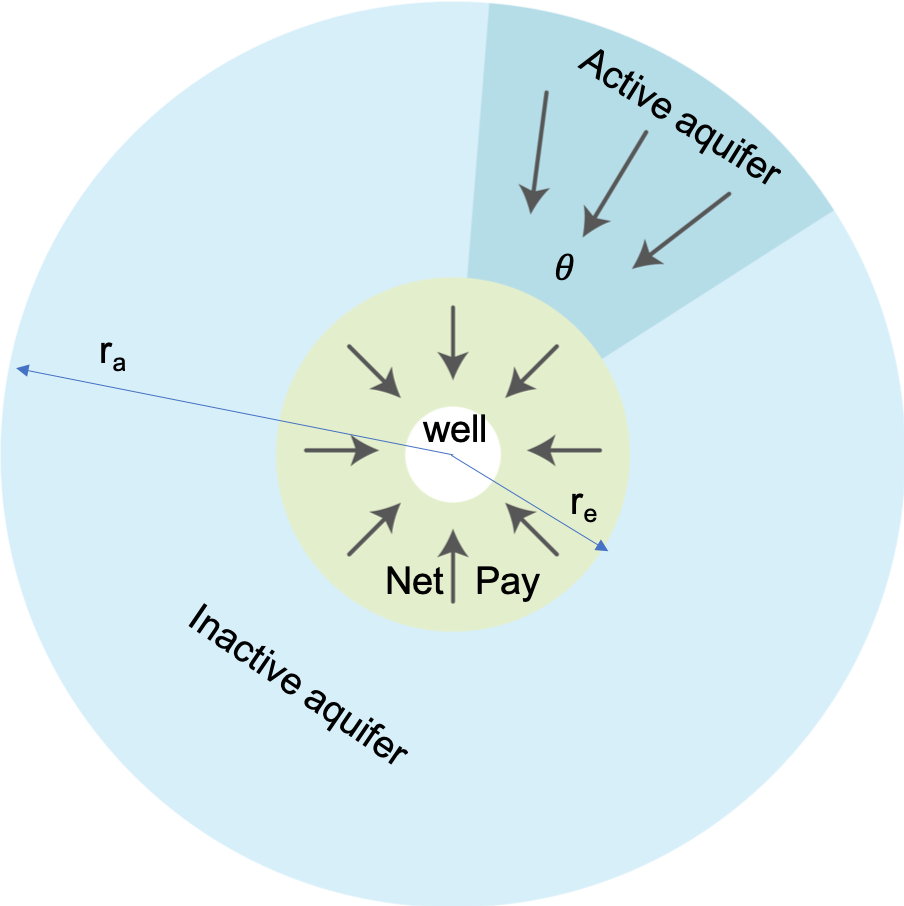
The Carter–Tracy (1960) model is a finite aquifer influx analytical model widely used in reservoir engineering to account for water influx in material-balance calculations.

It approximates the van Everdingen–Hurst (1949) solution fore faster computation.

Physical Model

Radial Composite Reservoir
Transient flow
Computational approximation to van Everdingen-Hurst (VEH)

	Fig. 1. Carter-Tracy aquifer drive schematic

Inputs

$\begin{array}{l}t\end{array}$	elapsed time
$\begin{array}{l}\mu\end{array}$	aquifer viscosity	$\begin{array}{l}h\end{array}$	aquifer thickness
$\begin{array}{l}k\end{array}$	aquifer permeability	$\begin{array}{l}r_e\end{array}$	inner radius (reservoir–aquifer interface)
$\begin{array}{l}\phi\end{array}$	aquifer porosity	$\begin{array}{l}r_a\end{array}$	outer radius of aquifer
$\begin{array}{l}c_\phi\end{array}$	aquifer pore compressibility	$\begin{array}{l}p_i\end{array}$	initial formation pressure
$\begin{array}{l}c_w\end{array}$	aquifer water compressibility	$\begin{array}{l}p(t)\end{array}$	field-average formation pressure at time moment $\begin{array}{l}t\end{array}$

Outputs

$\begin{array}{l}Q^{\downarrow}_{AQ}(t)\end{array}$	Cumulative subsurface water influx from aquifer at time $\begin{array}{l}t\end{array}$ , also denoted as $\begin{array}{l}W_e(t)\end{array}$
$\begin{array}{l}q_{AQ}^{\downarrow}(t)=\frac{Q^{\downarrow}_{AQ}(t)}{dt}\end{array}$	Subsurface water flowrate from aquifer

Midputs

$\begin{array}{l}A_e = \pi \, r_e^2\end{array}$	net pay area
$\begin{array}{l}c_t=c_\phi +c_w\end{array}$	aquifer total compressibility (fluid + rock)
$\begin{array}{l}B = \frac{\theta}{\pi} \cdot A_e \cdot h \cdot \phi \cdot c_t\end{array}$	water influx constant
$\begin{array}{l}\chi = \frac{ k }{\phi \, \mu \, c_t }\end{array}$	aquifer diffusivity
$\begin{array}{l}t_D = \frac{\pi \, \chi \, t}{A_e} = \frac{ k \, t}{\phi \, \mu \, c_t \, r_e^2}\end{array}$	dimensionless time
$\begin{array}{l}r_D=r_a/r_e\end{array}$	dimensionless radius of aquifer
$\begin{array}{l}F(t_D, r_D)\end{array}$	dimensionless water influx function (solution of Carter–Tracy PDE)

Mathematical Model

(1)	$\begin{array}{l}\displaystyle Q^{\downarrow}_{AQ}(t) = B \cdot \big( p_i- p(t) \big) \cdot F(t_D, r_D)\end{array}$

(2)	$\begin{array}{l}\displaystyle p_D(t_D)= \sum_{n=1}^\infty\frac{2 \, \cdot \left[ 1- \exp(-\alpha_n^2 \, t_D) \right]}{\alpha_n^2 \, J^2_1(\alpha_n)}\end{array}$

(3)	$\begin{array}{l}\displaystyle F(t_D,r_D)=\frac{p_D(t_D)}{\ln(r_D)}\end{array}$

where

$\begin{array}{l}J_1\end{array}$	first-order Bessel function
$\begin{array}{l}\alpha_n\end{array}$	roots of the zero-order Bessel function $\begin{array}{l}J_0(\alpha_n \, r_D)=0\end{array}$

Computational Model

(4)	$\begin{array}{l}\displaystyle p_D(t_D)\approx \frac{a_0 + a_1 z + a_2 z^2 + a_3 z^3 + a_4 z^4 + a_5 z^5 + a_6 z^6 + a_7 z^7 + a_8 z^8}{1 + b_1 z + b_2 z^2 + b_3 z^3 + b_4 z^4 + b_5 z^5 + b_6 z^6 + b_7 z^7 + b_8 z^8}\end{array}$

$\begin{array}{l}z=\frac{\sqrt{t_D}}{100}\end{array}$

where

a_{0} = 9.61160410 \times 1 0^{-5}

$b_{1} = 7.55537131 \times 1 0^{1}$

Reference

1. Carter, R.D. and Tracy, G.W. 1960. An Improved Method for Calculating Water Influx. Trans., AIME 219: 415.

2. Tarek Ahmed, Paul McKinney, Advanced Reservoir Engineering (eBook ISBN: 9780080498836)

Page tree

Motivation

Physical Model

Inputs

Outputs

Midputs

Mathematical Model

See Also

Reference

Page tree

Carter-Tracy Aquifer Drive @model

Motivation

Physical Model

Inputs

Outputs

Midputs

Mathematical Model

See Also

Reference