Motivation
The most accurate way to simulate Aquifer Expansion (or shrinkage) is full-field 3D Dynamic Flow Model where Aquifer Expansion is treated as one of the fluid phases and accounts of geological heterogeneities, gas fluid properties, relperm properties and heat exchange with surrounding rocks. Unfortunately, in many practical cases the detailed information on the aquifer is not available which does not allow a proper modelling of aquifer expansion using a geological framework. Besides many practical applications require only knowledge of cumulative water influx from aquifer under pressure depletion. This allows building an Aquifer Drive Models using analytical methods.
Inputs & Outputs
| Inputs | Outputs | ||
|---|---|---|---|
p(t) | field-average formation pressure at time moment t | Q^{\downarrow}_{AQ}(t) | Cumulative subsurface water influx from aquifer |
p_i | initial formation pressure | q^{\downarrow}_{AQ}(t) = \frac{dQ^{\downarrow}_{AQ}}{dt} | Subsurface water flowrate from aquifer |
B | water influx constant | ||
\chi | aquifer diffusivity | ||
A_e | net pay area | ||
Physical Model
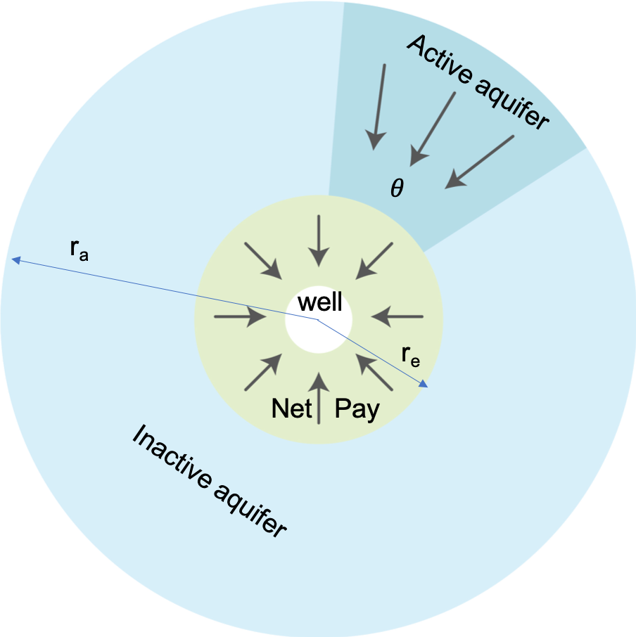
| Edge-water Drive Aquifer |
|
| Radial Composite Reservoir | |
| Transient flow | |
| Fig. 1. Radial VEH aquifer drive schematic |
Mathematical Model
|
|
|
| ||||||||||
|
|
|
or
|
Computational Model
|
This computational model is using a discrete convolution (also called superposition in some publications) with time-grid \{ \tau_1, \, \tau_2, \ ... \ , \tau_N \}.
In practical exercises with manual or spreadsheet-assisted calculations the time-grid is usually uniform: \{ \tau_1 =\Delta \tau, \, \tau_2 = 2 \cdot \Delta \tau, \ ... \ , \tau_N = N \cdot \Delta \tau\} with the time step \Delta \tau of a month to ensure the formation pressure does not change much since the previous time step.
Moving to annual time step may accumulate a substantial mistake if formation pressure has varied substantially in some years.
Scope of Applicability
The benefit of VEH approach is that net pay formation pressure history p(t) is usually known so that water influx calculation based on aquifer properties \{ B, \, r_a, \, \chi \} is rather straightforward.
In the past the VEH approach was considered as tedious in calculating superposition during the manual exercises.
In modern computers the convolution is a fast fully-automated procedure and VEH model is considered as a reference in the range of analytical aquifer models.
Although the model is derived for linear and radial flow it also shows a good match for bottom-water drive depletions.
See Also
Petroleum Industry / Upstream / Subsurface E&P Disciplines / Field Study & Modelling / Aquifer Drive / Aquifer Drive Models
Reference
1. van Everdingen, A.F. and Hurst, W. 1949. The Application of the Laplace Transformation to Flow Problems in Reservoirs. Trans., AIME 186, 305.
2. Tarek Ahmed, Paul McKinney, Advanced Reservoir Engineering (eBook ISBN: 9780080498836)
3. Klins, M.A., Bouchard, A.J., and Cable, C.L. 1988. A Polynomial Approach to the van Everdingen-Hurst Dimensionless Variables for Water Encroachment. SPE Res Eng 3 (1): 320-326. SPE-15433-PA. http://dx.doi.org/10.2118/15433-PA