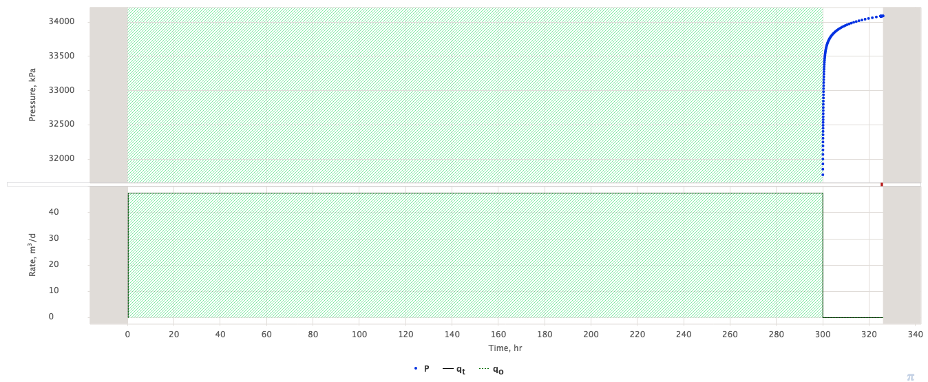
Specific schematic of Pressure Test consisting of long-term shut-in, followed by FLOWING survey (Drawdown / Injection) then followed by SHUT-IN survey(Build-up / Fall-off) (see Fig. 1).
|
| Fig. 1 – Horner Test schematic |
The interpretation of Horner Test can be performed by conventional pressure diffusion models fitting.
But historically it was given a specific popularity due to computational simplifications from using the Superposition Time concept, particularly when the following conditions hold true:
| Condition 1 | |
|---|---|
| Condition 2 |
In this case the pressure diffusion during the SHUT-IN period can be simulated as:
| (1) | p_{wf}(\Delta t) = p_e - \frac{q_t}{4 \pi \sigma} \, \ln \left( 1 + \frac{T}{\Delta t} \right) |
The equation (1) shows that pressure during this period of time is not dependent on skin-factor S and pressure diffusivity \chi but provide an easy linear way to assess formation pressure p_e and formation transmissibility \sigma.
The benefits of this interpretation method is that:
- it provides the robust straightforward estimation of formation pressure p_e and formation transmissibility \sigma
- it does not require the knowledge of pressure diffusivity \chi
- it does not depend on diffusion model specifics as soon as IARF is developed during the test and the outer boundary did not affect the pressure
It should be mentioned that in modern Pressure Transient Analysis the above Condition 1 and Condition 2 are not required and one can use the powerful arsenal of modern softwares to fit the pressure readings with pressure diffusion models.
See Also
Petroleum Industry / Upstream / Subsurface E&P Disciplines / Well Testing / Pressure Testing / Pressure Transient Analysis (PTA)