...
| LaTeX Math Block |
|---|
|
\bar q_t(t) = \frac{1}{Q} \int_0^t q^2_t(\tau) d\tau |
where
| LaTeX Math Inline |
|---|
body | | production/injection time |
| |
| |
|
\tau |
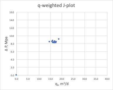 Image Modified Image Modified
|
Fig. 1 |
.4
It shows unit slope on log-log plot for stabilized reservoir flow:
...
Due to integration procedure the q-weighted J-plot has a better tolerance to uncertainties in formation pressure and bottomhole pressure comparing to Unweighted J-plot and usually results in more accurate estimation of productivity index.
It is highly recommended to plot sandface flowrates rather than surface flowrates to achieve better linearity in correlation for stabilized reservoir flow.
...
The main difference between q-weighted J-plot and t-weighted J-average and Normalized Hall Plotplot is the averaging methodology.
The Normalized Hall Plott-weighted J-plot gives equal weight to all data points
| LaTeX Math Inline |
|---|
| body | --uriencoded--\displaystyle w(t) = \frac%7B1%7D%7Bt%7D |
|---|
|
, while
q-weighted J-plot gives more weight to higher
flowrate data points, lower weight to lower
flowrate data points and zero weight to no-flow data points (
):
| LaTeX Math Inline |
|---|
| body | --uriencoded--\displaystyle w(t) = \frac%7Bq_t%7D%7BQ%7D |
|---|
|
.
When flowrate is constant
both methods are equivalent because
| LaTeX Math Inline |
|---|
| body | --uriencoded--\displaystyle w(t) = \frac%7Bq_t%7D%7BQ%7D =\frac%7B1%7D%7Bt%7D |
|---|
|
.
The q-weighted J-plot provides the same accuracy of productivity index estimation as Hall Plot but additionally provides a useful insight into the ranges of historically averaged flowrates and drawdowns.
See Also
...
Petroleum Industry / Upstream / Production / Subsurface Production / Field Study & Modelling / Production Analysis / Productivity Diagnostics
...