Motivation
In many practical cases the reservoir flow created by well is getting aligned with a radial direction towards or away from well.
This type of flow is called radial fluid flow and a type library model provides a reference for radial fluid flow diagnostics.
Physical Model
Mathematical Model
| Expand |
|---|
|
| LaTeX Math Block |
|---|
| \frac{\partial p}{\partial t} = \chi \, \left( \frac{\partial^2 p}{\partial r^2} + \frac{1}{r} \frac{\partial p}{\partial r} \right) |
|
| LaTeX Math Block |
|---|
| p(t = 0, {\bf r}) = p_i |
|
| LaTeX Math Block |
|---|
| p(t, r \rightarrow \infty ) = p_i |
|
| LaTeX Math Block |
|---|
| \frac{\partial p(t, r )}{\partial r} \bigg|_{r \rightarrow 0} = \frac{q_t}{\sigma \, d} |
|
|
| Expand |
|---|
|
| LaTeX Math Block |
|---|
| p(t,r) = p_i + \frac{q_t}{4 \pi \sigma} \, {\rm Ei} \bigg( - \frac{r^2}{4 \chi t} \bigg) |
|
| LaTeX Math Block |
|---|
| p_{wf}(t) = p_i + \frac{q_t}{4 \pi \sigma} \, \bigg[ - 2S + {\rm Ei} \bigg( - \frac{r_w^2}{4 \chi t} \bigg) \bigg] |
|
|
Scope of Applicability
See also
Physics / Fluid Dynamics / Radial fluid flow
[ Line Source Solution (LSS) @model ]
| Show If |
|---|
|
| Panel |
|---|
|
| Expand |
|---|
|
| Expand |
|---|
| | Include Page |
|---|
| Line Source Solution (LSS) |
|---|
| Line Source Solution (LSS) |
|---|
|
|
| LaTeX Math Block |
|---|
| p(t,r) = p_i + \frac{q_t}{4 \pi \sigma} \, {\rm Ei} \bigg( - \frac{r^2}{4 \chi t} \bigg) |
Рассмотрим плоскопараллельный аксиально-симметричный однородный пласт постоянной толщины , с радиальной координатой в перпендикулярной к оси скважины плоскости, который вскрыт бесконечно тонкой скважиной в точке (где – радиальная координата в перпендикулярной к оси скважине плоскости) и начальным пластовым давлением .
Пусть в момент времени
скважина запускается с дебитом (в пересчете на пластовые условия).Диффузия давления описывается решением уравнения однофазного радиального течения в бесконечном однородном пласте: | LaTeX Math Block |
|---|
| \frac{\partial p}{\partial t} = \chi \, \Delta p = \chi \, \frac{1}{r} \frac{\partial}{\partial r} \bigg( r \frac{\partial p}{\partial r} \bigg) |
с начальным условием: | LaTeX Math Block |
|---|
| p(t = 0, r) = p_i |
и граничными условиями: | LaTeX Math Block |
|---|
| p(t, r \rightarrow \infty ) = p_i |
| LaTeX Math Block |
|---|
| anchor | Boundary_q |
|---|
| alignment | left |
|---|
| r \frac{\partial p(t, x )}{\partial r} \bigg|_{r \rightarrow 0} = \frac{q_t}{2 \pi \sigma} |
где | LaTeX Math Inline |
|---|
| body | \sigma = \frac{k \, h}{\mu} |
|---|
|
– гидропроводность пласта, | LaTeX Math Inline |
|---|
| body | \chi = \frac{k}{\mu} \, \frac{1}{\phi \, c_t} |
|---|
|
– пьезопроводность пласта, – проницаемость пласта, – пористость пласта, – сжимаемость пласта, – сжимаемость порового коллектора, – сжимаемость насыщающего пласт флюида, – вязкость насыщающего пласт флюида.
При анализе отклика давления на самой скважине ( ) после включения на достаточно больших временах, удовлетворяющих условию:| LaTeX Math Block |
|---|
| t \gg \frac{r_w^2}{4 \chi}
|
которые на практике наступают очень быстро, можно воспользоваться приближением | LaTeX Math Inline |
|---|
| body | {\rm Ei}(-x) \sim \ln (x) + \gamma \sim \ln (1.781 x) |
|---|
|
, где – постоянная Эйлера.
Режим радиального течения к линейному источнику примет вид:
| LaTeX Math Block |
|---|
| p(t,r_w) = p_i + \frac{q_t}{4 \pi \sigma} \, \ln \bigg( 1.781 \, \frac{r_w^2}{4 \chi t} \bigg) |
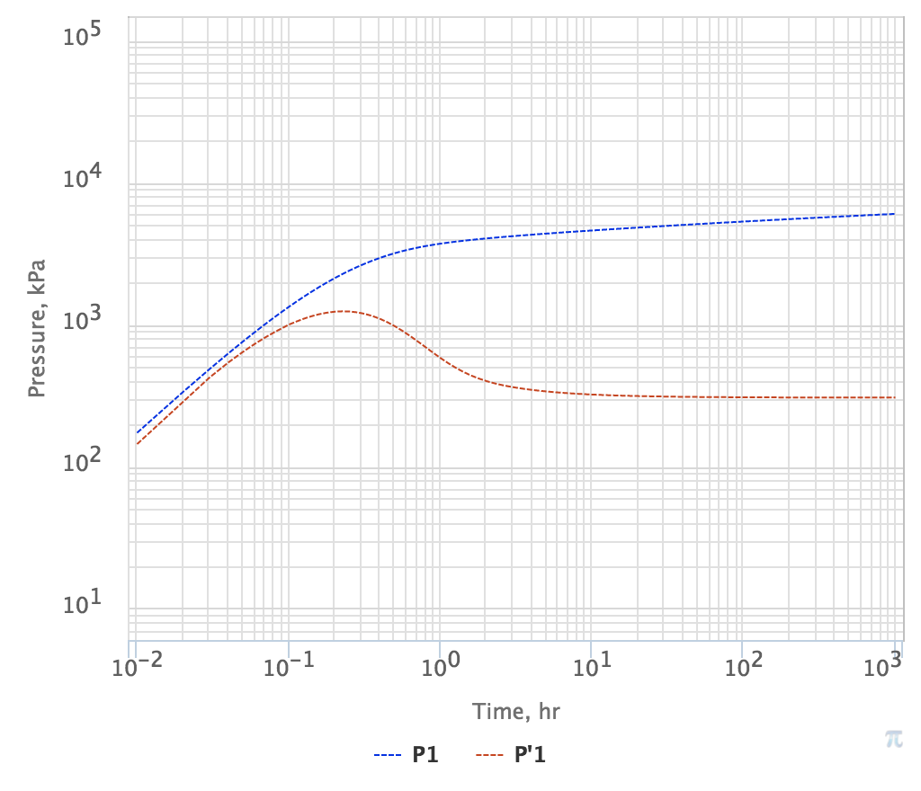
Отсюда следует, что уже вскоре после запуска скважины динамическая депрессия на пласт начинает логарифмически расти во времени:
| LaTeX Math Block |
|---|
| \delta p = p_i - p_{wf}(t) \sim { \rm const } + \frac{q_t}{4 \pi \sigma} \, \ln t |
а логарифмическая производная становится постоянной во времени: | LaTeX Math Block |
|---|
| t \frac{d (\delta p)}{dt} \sim \frac{q_t}{4 \pi \sigma} |
В лог-лог координатах лог-производная депрессии будет горизонтальной, что является характерным для радиальной фильтрации в бесконечном пласте.
|
|
|