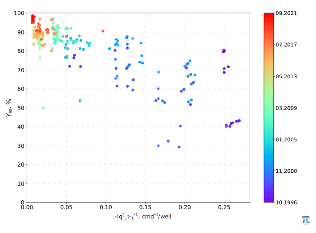
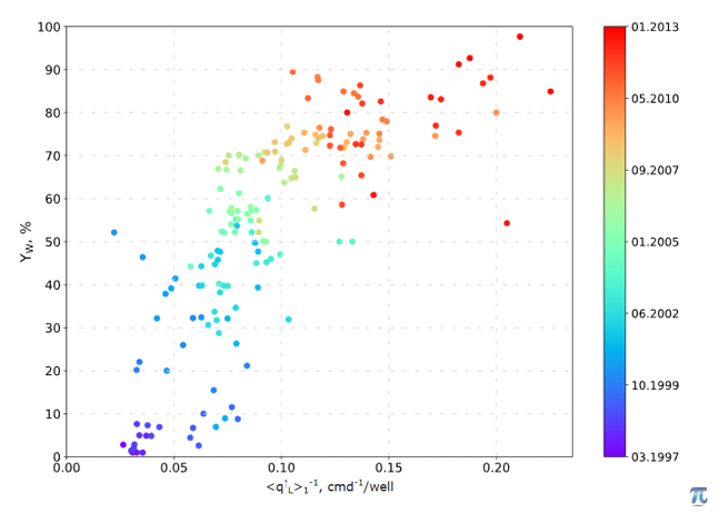
One if the Watercut Diagnostics plots with water cut (Yw) along y-axis and inverse liquid rate 1/q_L along x-axis (see Fig. 1 – Fig. 3).
|
|
|
| Fig. 1 – Good Water | Fig. 2 – Bad Water with low pressure | Fig. 3 – Bad Water with high pressure |
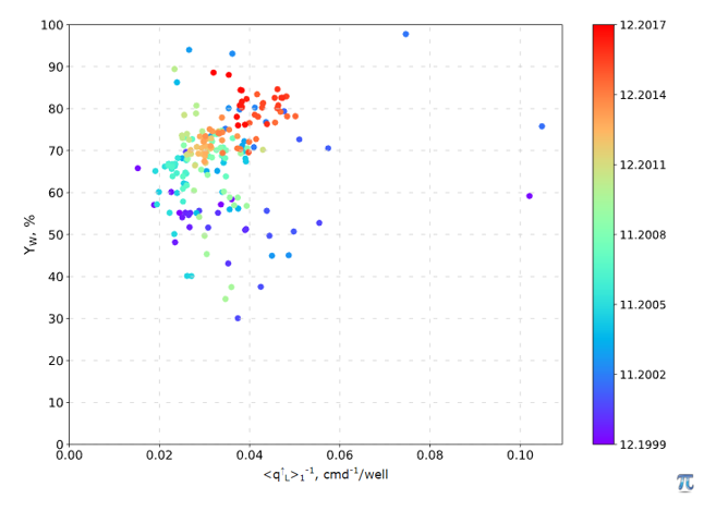
The absence of correlation between Yw and liquid rate suggest that either produced water is all good or it may have bad water production from the reservoir with the same formation pressure as oil pay: P_{\, {\rm bad} \, {\rm water}} = P_{{\rm oil} \, {\rm pay}} (see Fig. 1).
In practice, it is very rare occasion that bad water has the same formation pressure as the oil pay: P_{\, {\rm bad} \, {\rm water}} = P_{{\rm oil} \, {\rm pay}} and usually the absence of correlation between Yw and liquid rate indicates that all produced water is good.
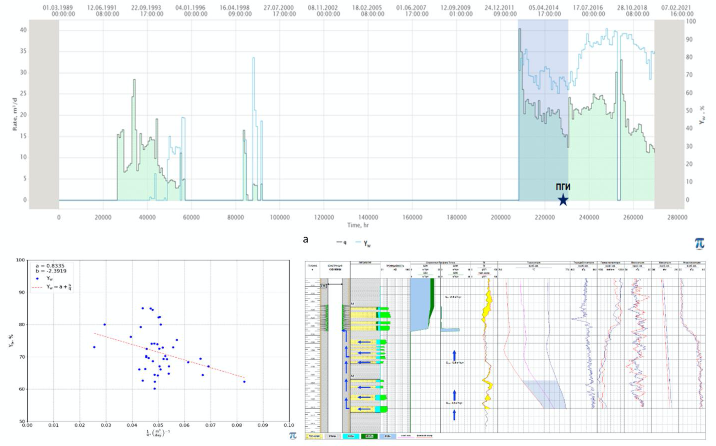
The negative correlation between Yw and inverse liquid rate 1/q_L suggests that produced water contains bad water with lower formation pressure than that of oil pay: P_{\, {\rm bad} \, {\rm water}} < P_{{\rm oil} \, {\rm pay}} (see Fig. 2).
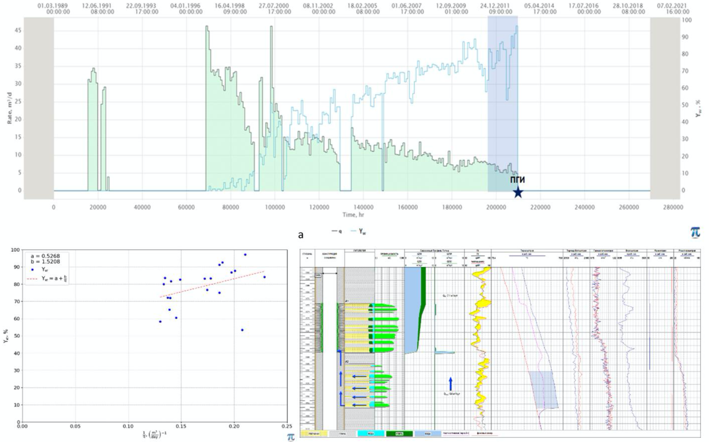
The positive correlation between Yw and inverse liquid rate 1/q_L suggests that produced water contains bad water with higher formation pressure than that of oil pay: P_{\, {\rm bad} \, {\rm water}} > P_{{\rm oil} \, {\rm pay}} (see Fig. 3).
There is no clear regulation on what value of correlation is enough to discriminate between the cases on Fig. 1 – Fig. 3.
This is usually done by an eye pick or artificial intelligence and stands as a part of the complex Watercut Diagnostics.
Some people see that growing Yw with increasing of liquid rate for low-pressure bad water is counter-intuitive but in reality this is a solid fact which can be easily verified mathematically and/or tested in practise.
The YLIQ analysis is not always applicable as sometimes well produces at constant rate and correlation with watercut can not be assessed.
But even when historical rates were varying the YLIQ analysis does not provide the unique answer on whether produced water contains bad water.
Nevertheless, in many practical cases YLIQ analysis is very helpful as additional argument (and sometimes as the key argument) in assessing if produced water contains bad water.
The mathematical model of the thief water production from aquifer is based on the following equation:
|
|
|
where
q_W | water production rate | q_L | liquid production rate | ||
p^*_1 | J_{1W} | water productivity index of petroleum reservoir | J_{1O} | oil productivity index of petroleum reservoir | |
p^*_2 | formation pressure in aquifer | J_{2W} | water productivity index of aquifer | ||
The equation (1) suggests that water cut declines along with aquifer pressure decline.
It also suggest that water cut grows with decline of the petroleum reservoir pressure and decreases when petroleum reservoir pressure grows.
For the case of aquifer pressure is higher than that of petroleum reservoir: b > 0 \Leftrightarrow p^*_2 > p^*_1,
which means that if aquifer pressure is higher than petroleum reservoir pressure then production increase will lead to the water cut decline.
For the case of aquifer pressure is lower than that of petroleum reservoir: b < 0 \Leftrightarrow p^*_2 < p^*_1,
which means that if aquifer pressure is lower than petroleum reservoir pressure then production increase will lead to the water cut growth.
In practical applications, the equation (1) is often considered through the weighted average values:
| (4) | Y_W = \frac{ \langle q_W \rangle}{\langle q_L \rangle} = a + b \, \cdot \langle q_L \rangle^{-1} |
where
\langle q_W \rangle, \ \langle q_O \rangle | are weighted average of q_W and q_O |
There are different ways to calculate weighted average of the dynamic variable, for example:
|
|
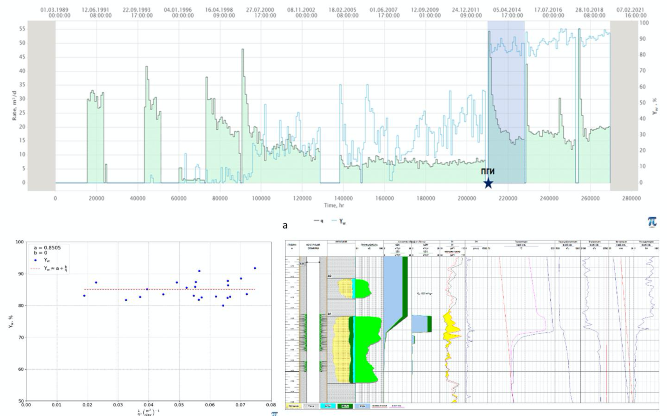
Cases
Case 1
|
| Fig. 4 – Good Water |
Case 2
|
| Fig. 5 – Bad Water with low pressure |
Case 3
|
| Fig. 6 – Bad Water with high pressure |
See Also
Petroleum Industry / Upstream / Production / Subsurface Production / Field Study & Modelling / Production Analysis / Watercut Diagnostics