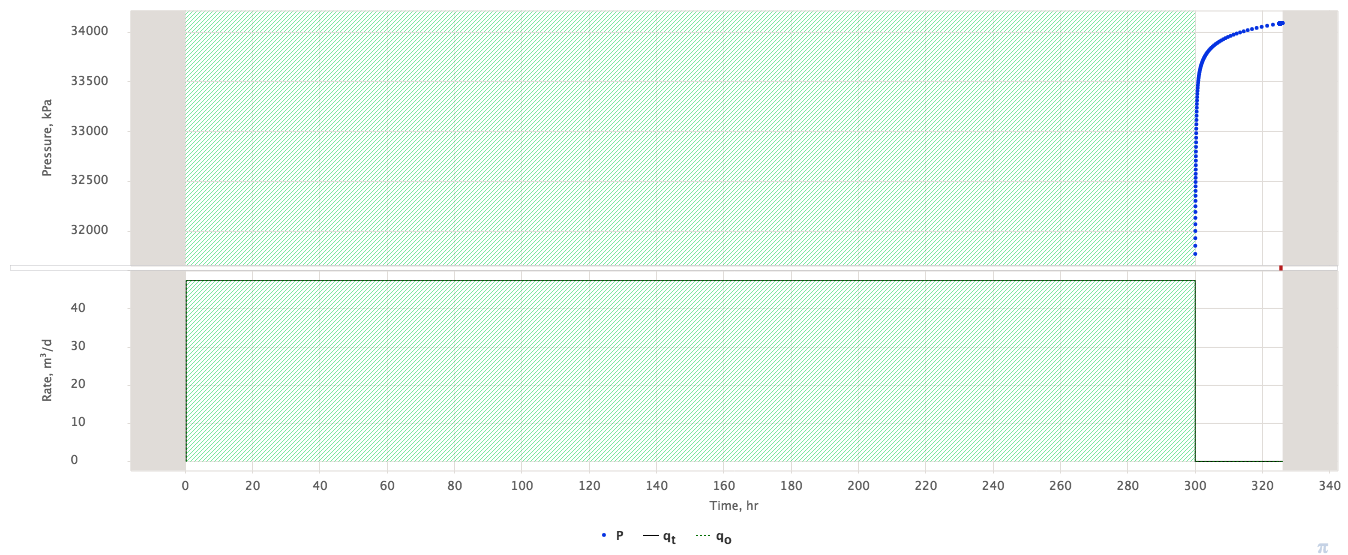
Specific schematic of Pressure Test consisting of long-term shut-in, followed by FLOWING test (Drawdown / Injection) then followed by Build-up / Fall-off (see Fig. 1).
|
| Fig. 1 – Horner Test schematic |
The interpretation of Horner Test can be performed by conventional pressure diffusion model fitting.
But historically it was given a specific focus due to simplifications from using the Superposition Time concept, particularly when the following conditions hold true:
- both production
T and shut-in
\Delta t period reach radial flow regime:
T > t_{IARF},
\Delta t > t_{IARF}
- total duration of production and shut-in do not reach the boundary T+\Delta t < t_e
In this case one
| (1) | p_{wf}(\Delta t) = p_e - \frac{q_t}{4 \pi \sigma} \, \ln \left( 1 + \frac{T}{\Delta t} \right) |
The main features of Horner model are:
it provides reliable estimation of formation pressure p_e and formation transmissibility \sigma
it does not require the knowledge of pressure diffusivity \chi (unlike the case of a drawdown test)
it does not depend on diffusion model specifics as soon as IARF is developed during the test
it does not provide skin-factor estimation
The formula (1) shows that pressure during the shut-in segment of Honer test is not dependant on skin-factor and pressure diffusivity.
The formation pressure p_e and transmissibility \sigma are estimated with LSQ regression:
| \left \{ p_{wf} \right \} = p_e - b \, \left \{ \ln \left( 1 + \frac{T}{\Delta t} \right) \right \} |
| \sigma = \frac{q_t}{4 \pi b} |
Horner model is a good example of how a complicated problem of non-linear regression on three parameters \{ p_e, \, S, \, \sigma \} with upfront knowledge of pressure diffusivity may sometimes be simplified to a fast-track linear regression on two parameters without any additional assumptions on reservoir properties.
See Also
Petroleum Industry / Upstream / Subsurface E&P Disciplines / Well Testing / Pressure Testing / Pressure Transient Analysis (PTA)