Interpretation of BUS in terms of formation pressure and formation transmissibility under the following (Horner) conditions:
Horner Conditions
both production T and shut-in t period reach radial flow regime: T > t_{IARF}, t > t_{IARF}
total duration of production and shut-in do not reach the boundary
T+t < t_e
|
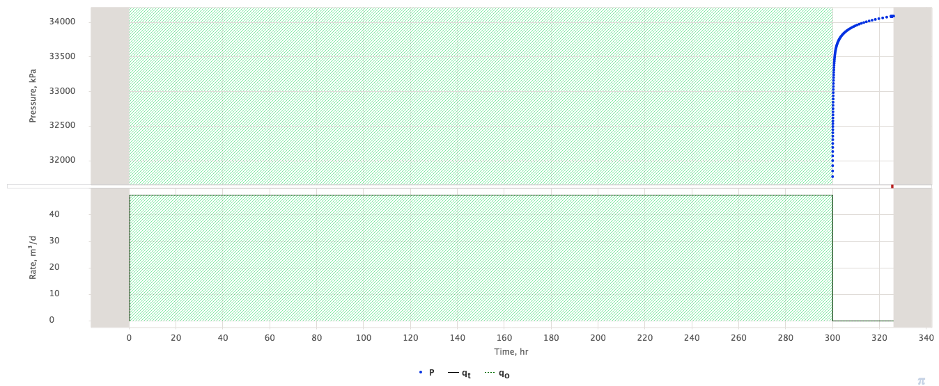
| Fig. 1. BUS with Horner conditions applied |
In some cases when:
both production T and shut-in \Delta t period reach radial flow regime: T > t_{IARF}, \Delta t > t_{IARF}
total duration of production and shut-in do not reach the boundary
T+\Delta t < t_e
one can uses Horner model which is a simplified version of BUS interpretation procedure and based on the following pressure diffusion model:
| (1) | p_{wf}(\Delta t) = p_e - \frac{q_t}{4 \pi \sigma} \, \ln \left( 1 + \frac{T}{\Delta t} \right) |
The main features of Horner model are:
it provides reliable estimation of formation pressure p_e and formation transmissibility \sigma
it does not require the knowledge of pressure diffusivity \chi (unlike the case of a drawdown test)
it does not depend on diffusion model specifics as soon as IARF is developed during the test
it does not provide skin-factor estimation
The formula (1) shows that pressure during the shut-in segment of Honer test is not dependant on skin-factor and pressure diffusivity.
The formation pressure p_e and transmissibility \sigma are estimated with LSQ regression:
| \left \{ p_{wf} \right \} = p_e - b \, \left \{ \ln \left( 1 + \frac{T}{\Delta t} \right) \right \} |
| \sigma = \frac{q_t}{4 \pi b} |
Horner model is a good example of how a complicated problem of non-linear regression on three parameters \{ p_e, \, S, \, \sigma \} with upfront knowledge of pressure diffusivity may sometimes be simplified to a fast-track linear regression on two parameters without any additional assumptions on reservoir properties.
Тест Хорнера относится к частному случаю двухрежимного нестационарного теста (2НТ), при котором скважину после длительной эксплуатации с постоянным дебитом q_{t1} в течении времени T отключают и регистрируют динамику забойного давления p_{wf}(t), где отсечет времени t ведется с момента остановки скважины. То есть по сути это это 2НТ с q_{t2}=0 (см. рисунок 3).
Из формулы
при q_{t2} = 0 следует:| (2) | p_{wf}(t) = p_e - \frac{q_t}{4 \pi \sigma} \, \left[ -2S + F \left( - \frac{r_w^2}{4 \chi (t - T)} \right) \right] + \frac{q_t}{4 \pi \sigma} \, \left[ - 2S - F \left( - \frac{r_w^2}{4 \chi t} \right) \right] |
Отсюда следует что транзиент давления на остановке не содержит сведения о скин-факторе.
Если однородный пласт полностью вскрыт вертикальной скважиной без трещин и на временах порядка времени наблюдения t граница не достигается, то диффузия происходит в режиме IARF и F(z) \sim \gamma + \ln(-z), откуда:
| (3) | p_{wf}(t) = p_e - \frac{q_t}{4 \pi \sigma} \, \bigg[ \gamma + \ln \bigg( - \frac{r_w^2}{4 \chi (t - T)} \bigg) - \gamma - \ln \bigg( - \frac{r_w^2}{4 \chi t} \bigg) \bigg] = p_e - \frac{q_t}{4 \pi \sigma} \, \ln \frac{t}{t-T} |
Отсюда видно, что в этом режиме течения влияние пьезопроводности на динамику давления Хорнер-теста полностью отсутствует и с помощью простого МНК в координатах \{ p_{wf}, \, \ln \frac{t}{t-T} \} легко находится пластовое давление на начало теста p_e и гидропроводность пласта \sigma.
Хорнер-тест является ярким примером того, как мультирежимный тест позволяет свести сложную задачу анализа транзиента и неоднозначного поиска в трехмерном пространстве \{ p_e, \, S, \, \sigma \} к последовательности простых прямых вычислительных процедур с однозначным результатом