Motivation

The most accurate way to simulate Aquifer Expansion (or shrinkage) is full-field 3D Dynamic Flow Model where Aquifer Expansion is treated as one of the fluid phases and accounts of geological heterogeneities, gas fluid properties, relperm properties and heat exchange with surrounding rocks.

Unfortunately, in many practical cases the detailed information on the aquifer is not available which does not allow a proper modelling of aquifer expansion using a geological framework.

Besides many practical applications require only knowledge of cumulative water influx from aquifer under pressure depletion.

This allows building an Aquifer Drive Models using analytical methods.

Inputs & Outputs

Inputs		Outputs
$\begin{array}{l}p(t)\end{array}$	field-average formation pressure at time moment $\begin{array}{l}t\end{array}$	$\begin{array}{l}Q^{\downarrow}_{AQ}(t)\end{array}$	cumulative subsurface water influx from aquifer
$\begin{array}{l}p_i\end{array}$	initial formation pressure	$\begin{array}{l}q^{\downarrow}_{AQ}(t) = \frac{dQ^{\downarrow}_{AQ}}{dt}\end{array}$	subsurface water flowrate from aquifer
$\begin{array}{l}J_{AQ}\end{array}$	aquifer Productivity Index
$\begin{array}{l}\displaystyle \tau = \frac{c_t \, V_\phi}{J_{AQ}}\end{array}$	aquifer relaxation time

Detailing

Detailing Inputs
$\begin{array}{l}\displaystyle J_{AQ} = \frac{\theta}{2\pi} \cdot \frac{2 \pi \sigma}{\ln \frac{A_{AQ}}{A_e}+0.75}\end{array}$	aquifer Productivity Index
$\begin{array}{l}\theta\end{array}$	central angle of net pay area ↔ aquifer contact
$\begin{array}{l}\sigma\end{array}$	aquifer transmissibility
$\begin{array}{l}A_e\end{array}$	net pay area
$\begin{array}{l}A_{AQ}\end{array}$	aquifer area
$\begin{array}{l}\displaystyle \tau = \frac{V_{AQ} \, c_t}{J_{AQ}}\end{array}$	aquifer relaxation time
$\begin{array}{l}c_t=c_r +c_w\end{array}$	aquifer total compressibility
$\begin{array}{l}c_r\end{array}$	aquifer pore compressibility
$\begin{array}{l}c_w\end{array}$	aquifer water compressibility
$\begin{array}{l}V_{AQ} = A_e \cdot h \cdot \phi\end{array}$	aquifer volume
$\begin{array}{l}h\end{array}$	aquifer effective thickness
$\begin{array}{l}\phi\end{array}$	aquifer porosity

Physical Model

Radial Composite Reservoir

Const Productivity Index Aquifer

$\begin{array}{l}\displaystyle J_{AQ} = \frac{q_{AQ}}{p_{AQ}(t)-p(t)} = \rm const\end{array}$

Pseudo Steady State Flow

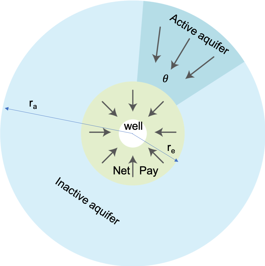
$\begin{array}{l}\displaystyle p_{AQ}(t) = p_i - \frac{Q_{AQ}(t)}{V_{AQ} \cdot c_t}\end{array}$

Fig. 1. Fetkovich aquifer drive schematic

Mathematical Model

(1)	$\begin{array}{l}\displaystyle \tau \cdot \frac{d Q^{\downarrow}_{AQ}}{dt} + Q^{\downarrow}_{AQ} = с_t \, V_\phi \cdot \left[ p_i - p(t) \right]\end{array}$

(2)	$\begin{array}{l}\displaystyle q^{\downarrow}_{AQ}(t)=\frac{d Q^{\downarrow}_{AQ}}{dt}\end{array}$

which can be explicitly integrated:

(3)	$\begin{array}{l}\displaystyle Q^{\downarrow}_{AQ}(t) = J_{AQ} \, \exp \left( -\frac{t}{\tau} \right) \, \int_0^t \big[ p_i - p(\xi) \big] \, \exp \left( \frac{\xi}{\tau} \right) \, d \xi\end{array}$

Derivation

Assumption #1 = Const Productivity Index Aquifer:

$\begin{array}{l}\displaystyle q_{AQ} = \frac{d Q_{AQ}}{dt} = J_{AQ} \cdot ( p_{AQ}(t) - p(t))\end{array}$

Assumption #2 = Pseudo Steady State Flow:

$\begin{array}{l}\displaystyle p_{AQ}(t) = p_i - \frac{Q_{AQ}}{c_t \, V_\phi}\end{array}$

Eliminating $\begin{array}{l}p_{AQ}(t)\end{array}$ one arrives to (1).

Reference

1. Fetkovich, M.J. 1971. A Simplified Approach to Water Influx Calculations—Finite Aquifer Systems. J Pet Technol 23 (7): 814–28. SPE-2603-PA. http://dx.doi.org/10.2118/2603-PA

Page tree

Motivation

Inputs & Outputs

Physical Model

Mathematical Model

See Also

Reference

Page tree

Fetkovich Aquifer Drive @model

Motivation

Inputs & Outputs

Physical Model

Mathematical Model

See Also

Reference