You are viewing an old version of this page. View the current version.
Compare with Current
View Page History
« Previous
Version 216
Next »
Definition
Primary Production Analysis is the specific workflow and report template on Primary Well & Reservoir Performance Indicators.
Application
- Assess current production performance
- current distribution of recovery against expectations
- current status and trends of recovery against expectations
- current status and trends of reservoir depletion against expectations
- current status and trends of water flood efficiency against expectations
- compare performance of different wells or different groups of wells
- Identify and prioritize surveillance opportunities
- Identify and prioritize redevelopment opportunities
Technology
Primary Production Analysis is built around production data against material balance and require current FDP volumetrics, PVT and SCAL models.
The PRIME workflow has certain specifics for oil producers, water injectors, gas injectors and field/sector analysis.
The PRIME analysis is
- fast-track
- based on the most robust input data
- does not involve full-field 3D dynamic modelling and associtated assumptions
Obviously, PRIME does not pretend to predict pressure and reserves distribution as 3D dynamic model does.
It only provides hints for misperoforming wells and sectors which need a further focus.
PRIME Metrics
| Metric name | Diagnostic plots | Objectives |
|---|
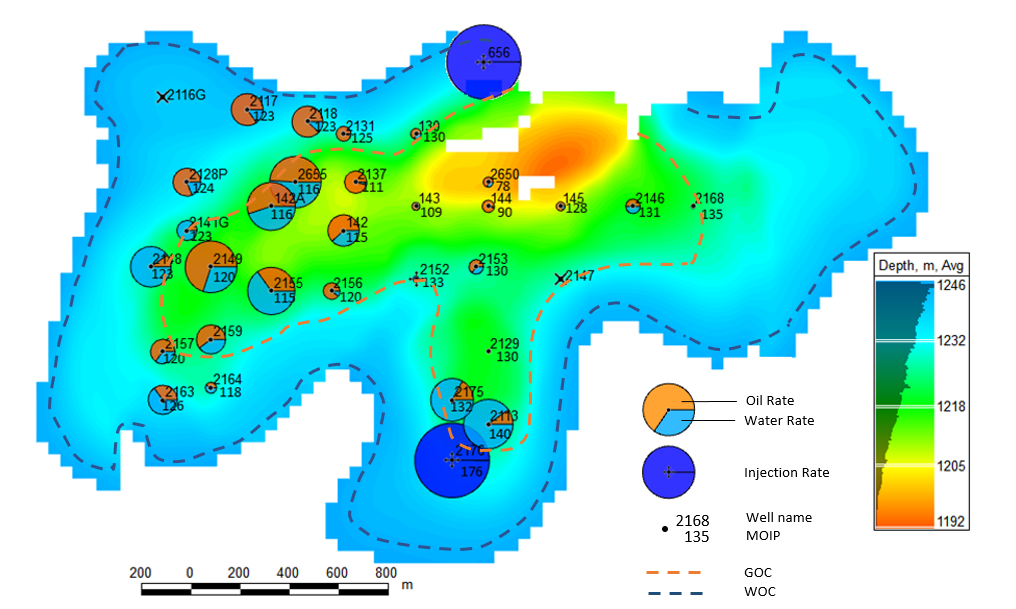
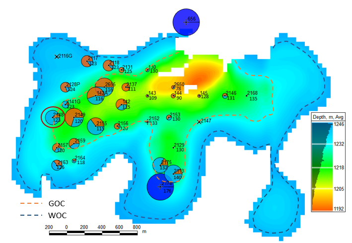
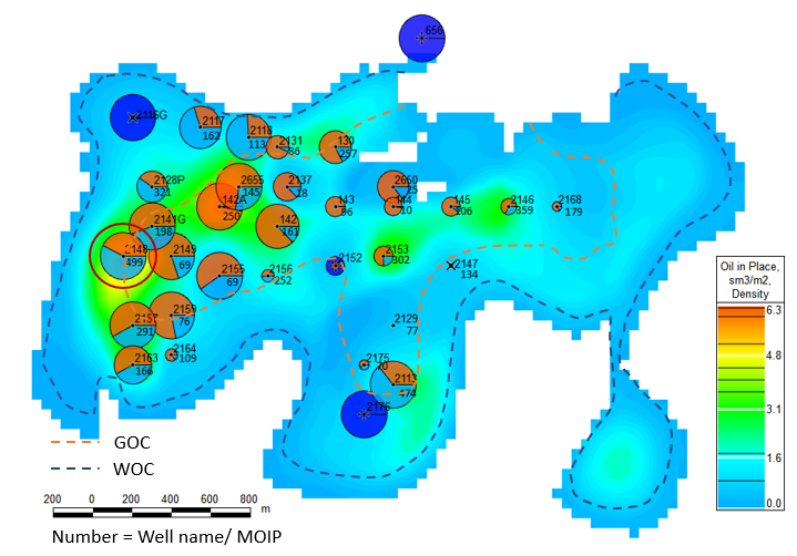
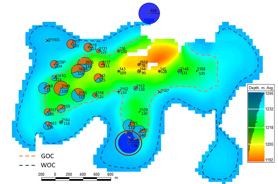
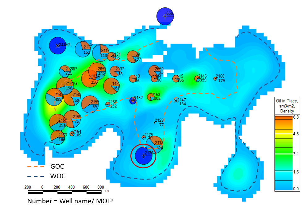
| 1 | Production History Map | Background = Structure Bubbles = qo, qg , qw, qinj Number = CurVRR, Pe | Production Distribution Overview |
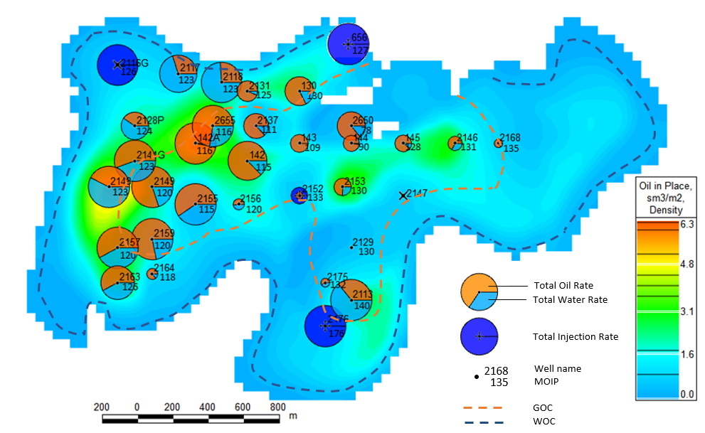
| 2 | Recovery Map | Background = STOIIP Bubbles = Qo, Qg , Qw, Qinj Number = CumVRR, Pe | Recovery Distribution Overview |
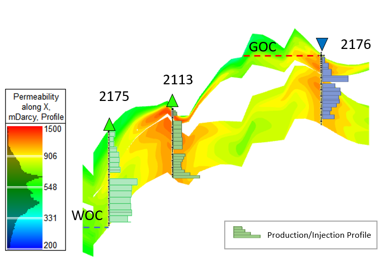
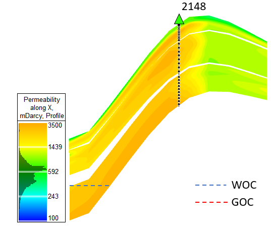
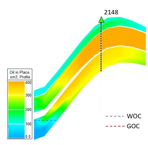
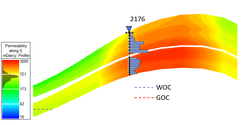
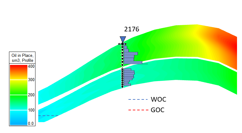
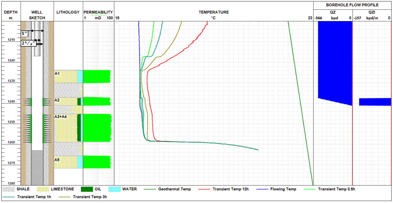
| 3 | Cross-section | Background = STOIIP & Structure Bubbles = VRR Number = Pe , Pem | Vertical Flow Proifle Overview |
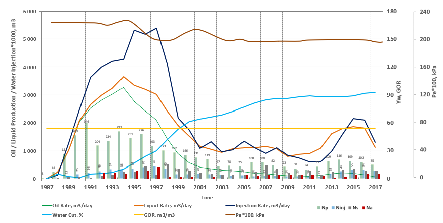
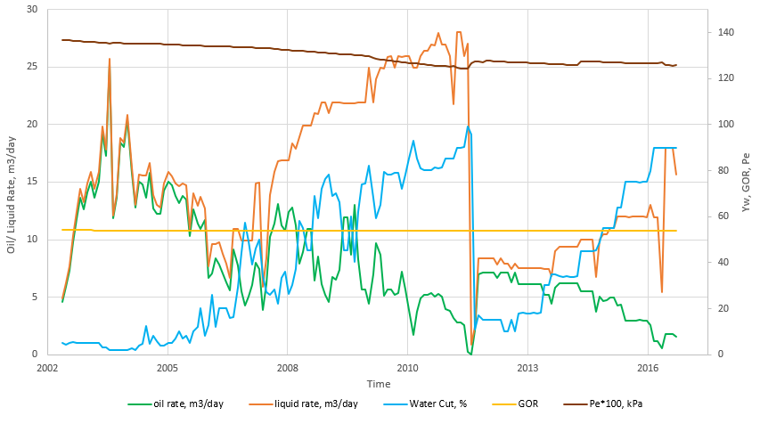
| 3 | Production History Graphs | Left Axis = qo, qg , qw, qinj, Rigth Axis = Yw, GOR, Pe , Np, Ninj Hor Axis = Elapsed Time | Production History Overview |
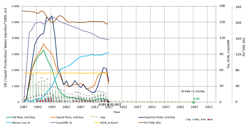
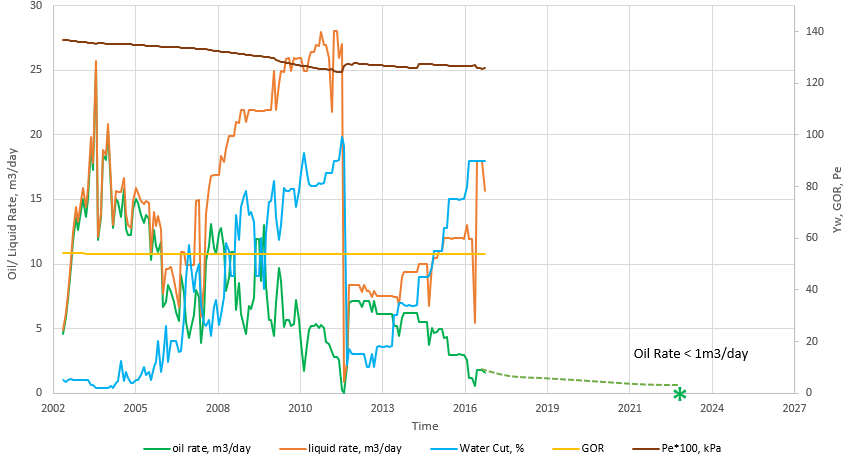
| 4 | Decline Curve Analysis | Left Axis = qo1, qliq1, qinj1, Rigth Axis = Yw, GOR, VRR, Pe
Hor Axis = Elapsed Time | Production Forecast |
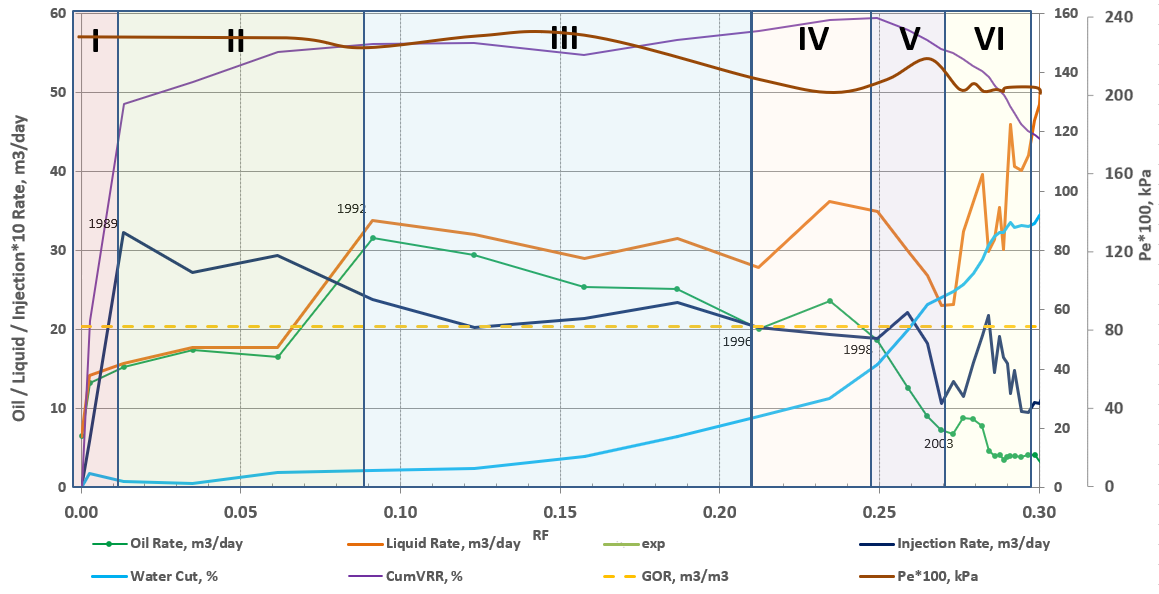
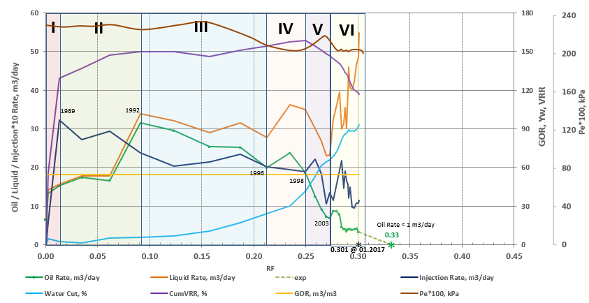
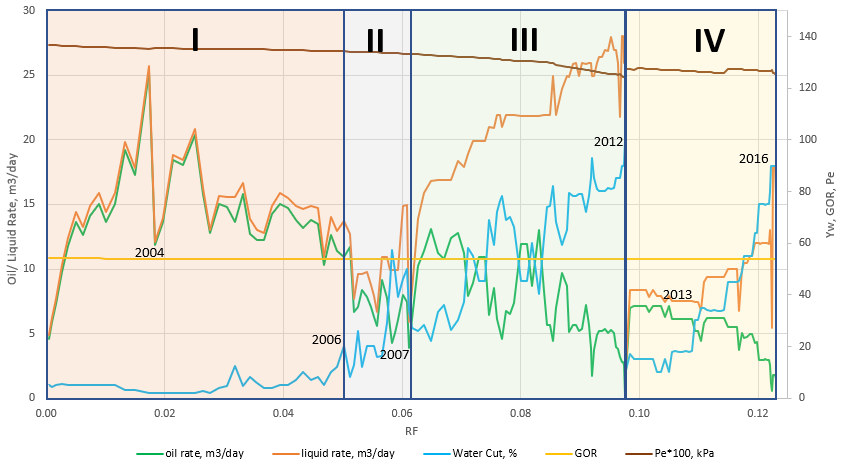
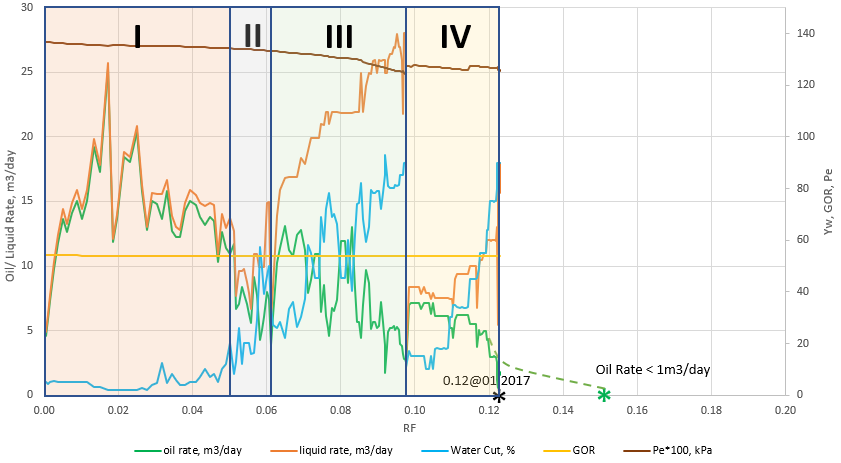
| 5 | Recovery Diagnostic | Left Axis = qo1, qliq1, qinj1 Rigth Axis =Yw, GOR, VRR, Pe, Pem
Hor Axis = RF | Estimate recovery efficiency and pressure decline |
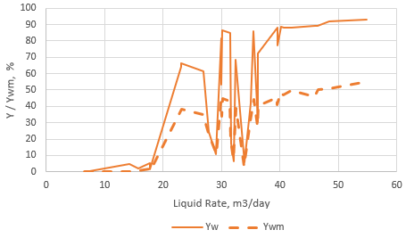
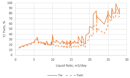
| 6 | Watercut Diagnostic | Left Axis = Yw, Ywm
Hor Axis = qliq | Check for water balance and thief water production |
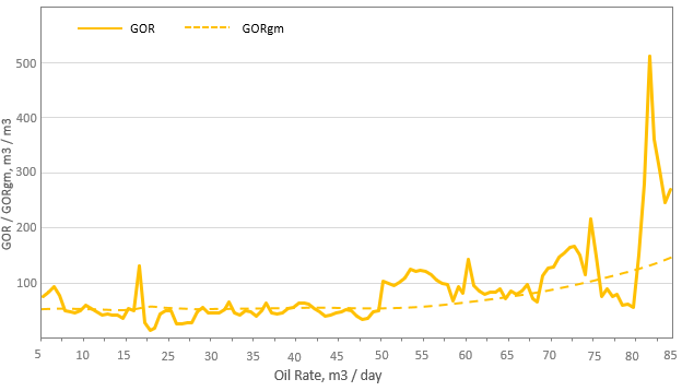
| 7 | GOR Diagnostic | Left Axis = GOR, GORgm Hor Axis =qo | Check for gas balance and thief gas production |
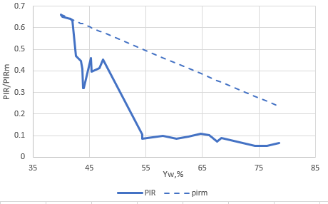
| 8 | Injection Efficiency Diagnostics | Left Axis = PIR , PIRm Hor Axis = Yw | Evaluate WI efficiency |
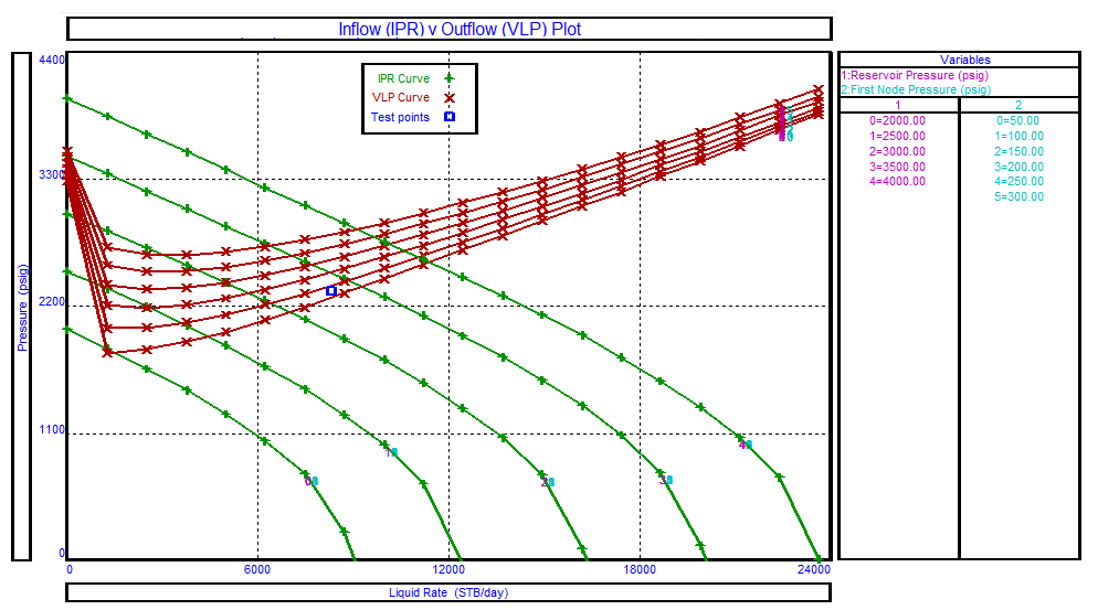
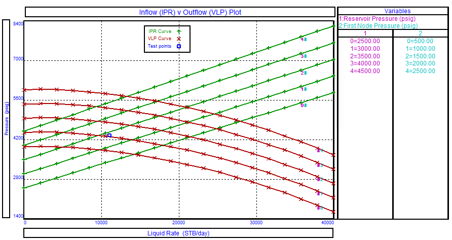
| 9 | Well Performance Analysis | Left Axis = Pwf_IPR , Pwf_VLP Hor Axis = qo | Check for the optimal production/injection target |
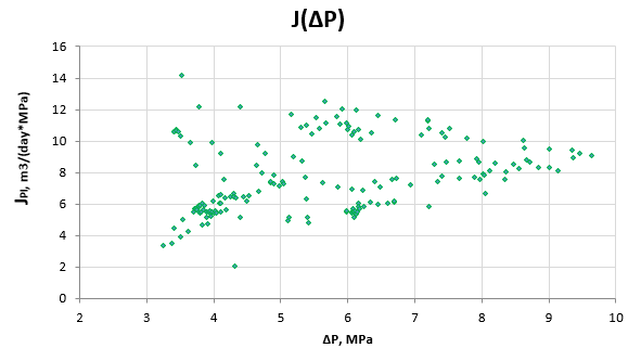
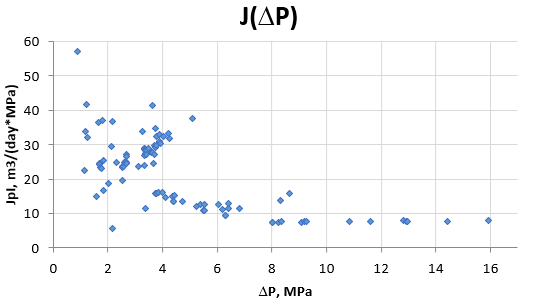
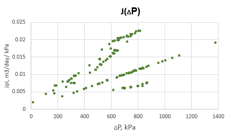
| 10 | Productivity Index Diagnostic | Left Axis = JPI, JPIm Hor Axis = dP = Pwf - Pe | Check for PI dynamics |
PRIME Mathematics
| Property Abbrevy | Property Name | Formula |
|---|
| VRRcum | Cumulative Voidage Replacement Ratio |
| (1) |
{\rm VRR_{cum}} = \frac{B_w \, Q_{WI}}{B_w \, Q_W + B_o \, Q_O + B_g Q_G - B_g R_s Q_O} |
|
| VRRcur | Current Voidage Replacement Ratio (month over month) |
| (2) |
{\rm VRR_{cur}} = \frac{B_w \, q_{WI}}{B_w \, q_W + B_o \, q_O + B_g (q_G - R_s Q_O)} |
|
| RF | Recovery Factor
|
| (3) |
{\rm RF} = \frac{Q_O}{V_{STOIIP}} |
|
| Yw | Watercut (production) |
| (4) |
{\rm Y_w} = \frac{q_W}{q_{LIQ}} |
|
| Ywm | Watercut (proxy-model) |
| (5) |
{\rm Y_{wm}} = \frac{1}{1 + \frac{K_{ro}}{K_{rw}} \cdot \frac{ \mu_w}{\mu_o} \cdot \frac{B_w}{B_o} } |
| (6) |
s_w = \frac{Q_o \, B_o}{V_\phi} |
|
| GOR | Gas-Oil Ratio (production) |
| (7) |
{\rm GOR} = \frac{q_g}{q_o} |
|
| GOR_m | Gas-Oil Ratio (proxy-model) |
| (8) |
{\rm GOR_m} = R_s + \frac{k_{rg}}{k_{ro}}
\cdot \frac{\mu_o}{\mu_g}
\cdot \frac{B_o }{B_g} |
|
| qLIQ | Liquid rate | |
PIR | Production Injection Ratio (production)
|
| (10) |
{\rm PIR} = \frac{Q_O}{Q_{WI}} |
|
| PIRm | Production Injection Ratio (model) |
| (11) |
{\rm PIR_m} = { \frac{1}{VRR} } \cdot { \frac{1-Y_w}{ Y_w + (1-Y_w) \bigg[ \frac{B_o}{B_w} - \frac{B_g}{B_w}(GOR - R_s) \bigg] } } |
|
| JO | Oil Productivity Index |
| (12) |
{\rm J_{O}} = \frac{q_O}{P_e - P_{wf}} {\quad \Rightarrow \quad} P_{wf} = P_e - \frac{1}{J_O} q_O |
|
JPI | Total Productivity Index (production)
|
| (13) |
{\rm J_t} = \frac{q_t}{P_e - P_{wf}} |
|
| JPIm | Total Productivity Index (model) |
| (14) |
{\rm J_{tm} } = \frac{2 \pi \sigma}{\ln \frac{r_e}{r_w} +0.5 + S} |
|
| jPI | Total Specific Productivity Index |
| (15) |
{\rm j_t} = \frac{q_t}{h \cdot (P_e - P_{wf})} |
|
| jPIm | Total Specific Productivity Index (model) |
| (16) |
{\rm j_{tm} } = \frac{2 \pi <k/\mu>}{\ln \frac{r_e}{r_w} +0.5 + S} |
|
Derivation of PIR equation
| (17) |
VRR = \frac{B_w \, q_{WI}}{B_w \, q_W + B_o \, q_O + B_g \, [ q_G - R_s \, q_O] } = \frac{B_w \, q_{WI}}{B_w \, q_W + B_o \, q_O + B_g \, [ GOR - R_s] q_O } = \frac{B_w \, q_{WI}}{B_w \, q_W + [ B_o + B_g \, ( GOR - R_s) ] \, q_O } |
| (18) |
VRR = \frac{q_{WI}}{q_W + \bigg[ \frac{B_o}{B_w} + \frac{B_g}{B_w} \, ( GOR - R_s) \bigg] \, q_O } |
| (19) |
Y_w=\frac{q_W}{q_W + q_O} \rightarrow \frac{q_O}{q_W} = \frac{1-Y_w}{Y_w} \rightarrow q_W = \frac{Y_w}{1-Y_w} \, q_O |
| (20) |
VRR = \frac{q_{WI}}{q_O} \cdot \frac{1}{\frac{Y_w}{1-Y_w} + \bigg[ \frac{B_o}{B_w} + \frac{B_g}{B_w} \, ( GOR - R_s) \bigg] } =
\frac{q_{WI}}{q_O} \cdot \frac{1-Y_w}{Y_w + (1-Y_w) \, \bigg[ \frac{B_o}{B_w} + \frac{B_g}{B_w} \, ( GOR - R_s) \bigg] } |
| (21) |
PIR=\frac{q_W}{q_{WI}} = \frac{1}{VRR} \cdot \frac{1-Y_w}{Y_w + (1-Y_w) \, \bigg[ \frac{B_o}{B_w} + \frac{B_g}{B_w} \, ( GOR - R_s) \bigg] } |
› PRIME Diagnostics
Sample Case 1 – Waterflood Sector Analysis
| |
Fig. 1.1. | Fig. 1.2.
|
|
|
| |
| Fig. 2.1. | |
|
|
| |
| Fig. 3.2. |
|
|
| |
| Fig. 4.1. | Fig. 4.2. Recovery Forecasts |
|
|
|  |
| Fig. 5.1. | Fig. 5.2. |
|
|
| |
| Fig. 6.1. | Fig. 6.2. Specific I |
|
|
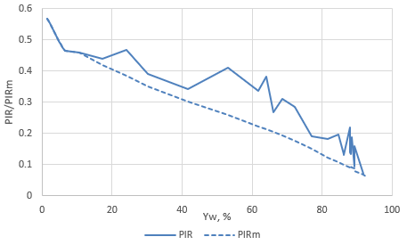 | |
Fig. 7. Injection Efficiency Diagnostics
|
|
Sample Case 2 – Oil Producer Analysis
| |
| Fig. 1.1 Production History Map | Fig. 1.2. Recovery Map |
|
|
| |
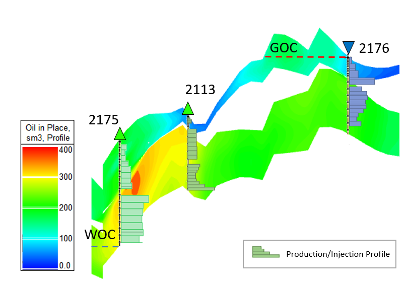
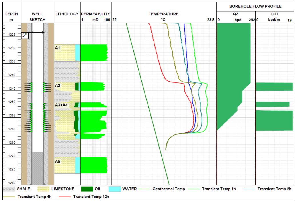
| Fig. 2.1. Cross-section & PLT, permeability, GOC, OWC | Fig. 2.2 Cross-section & PLT |
|
|
| |
| Fig. 3.1. Production History Graphs | Fig. 3.2. Decline Curve Analysis |
|
|
| |
| Fig. 4.1. Recovery Diagnostic | Fig. 4.2. Recovery Diagnostic |
|
|
| |
Fig. 5.1. Watercut Diagnostic | Fig. 5.2. GOR Diagnostic |
|
|
| |
| Fig. 6. Well Performance Analysis (VFP + IPR) | Fig. 7. Productivity Index Diagnostic |
|
|
| |
| Fig.8. Well Completion & PLT |
|
Sample Case 3 – Water Injector Analysis
| |
| Fig. 1.1. Production History Map | Fig. 1.2. Recovery Map |
|
|
| |
| Fig. 2.1. Cross-section & PLT | Fig. 2.2. Cross-section & PLT |
| |
| |
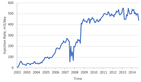
| Fig. 3.1. Injection History Graphs | Fig. 3.2. Injection Efficiency Diagnostics |
|
|
| |
| Fig. 4. Well Performance Analysis (VFP + IPR) | Fig. 5. Injectivity Index Diagnostic |
|
|
|
|
| Fig. 6. Well Completion & PLT |
|