The plot of WOR (along y-axis) against the inverse oil production rate $\begin{array}{l}q_O\end{array}$ (along x-axis) (see Fig. 1).

Fig. 1. WOR (logarithmic vertical axis) vs inverse oil production rate (linear horizontal axis)

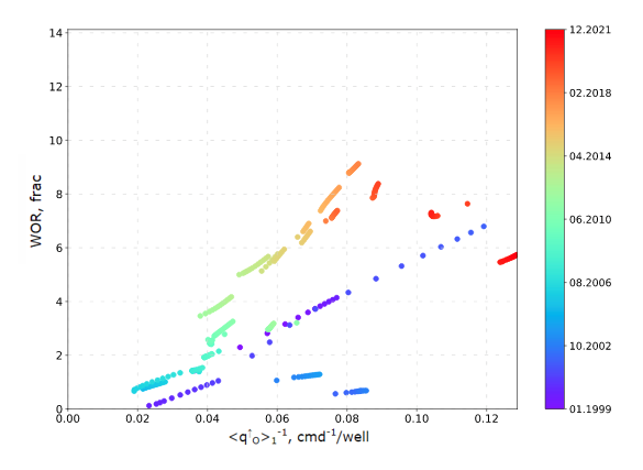
It can be used for express Watercut Diagnostics of thief water production.

The mathematical model of the thief water production from aquifer is based on the following equation:

(1)	$\begin{array}{l}\displaystyle WOR = \frac{q_W}{q_O} = a + b \, \cdot q^{-1}_O\end{array}$

(2)	$\begin{array}{l}\displaystyle a = J^{-1}_{1O} \cdot ( J_{1W} + J_{2W})\end{array}$

(3)	$\begin{array}{l}\displaystyle b = J_{2W} \cdot (p^_2 - p^_1)\end{array}$

where

		$\begin{array}{l}q_W\end{array}$	water production rate	$\begin{array}{l}q_O\end{array}$	oil production rate
$\begin{array}{l}p^*_1\end{array}$	formation pressure in petroleum reservoir	$\begin{array}{l}J_{1W}\end{array}$	water productivity index of petroleum reservoir	$\begin{array}{l}J_{1O}\end{array}$	oil productivity index of petroleum reservoir
$\begin{array}{l}p^*_2\end{array}$	formation pressure in aquifer	$\begin{array}{l}J_{2W}\end{array}$	water productivity index of aquifer

For the case of aquifer pressure is higher than that of petroleum reservoir: $\begin{array}{l}b > 0 \Leftrightarrow p^*_2 > p^*_1\end{array}$

For the case of aquifer pressure is lower than that of petroleum reservoir: $\begin{array}{l}b < 0 \Leftrightarrow p^*_2 < p^*_1\end{array}$

In practical applications, the equation (1) is often considered through the weighted average values:

(4)	$\begin{array}{l}\displaystyle \langle WOR \rangle =\frac{\langle q_W \rangle}{\langle q_O \rangle} = a + b \cdot \langle q_O^{-1} \rangle\end{array}$

where

$\begin{array}{l}\langle q_W \rangle, \ \langle q_O \rangle\end{array}$

are weighted average of $\begin{array}{l}q_W\end{array}$ and $\begin{array}{l}q_O\end{array}$

There are different ways to calculate weighted average of the dynamic variable, for example:

$\begin{array}{l}\displaystyle \langle A \rangle_t \ = \frac{1}{t} \int_o^t A(t) \, dt\end{array}$

$\begin{array}{l}\displaystyle \langle A\rangle_q \ = \frac{1}{Q(t)} \int_o^t A(t) \, q(t) \, dt\end{array}$

References

Page tree