...
...
|
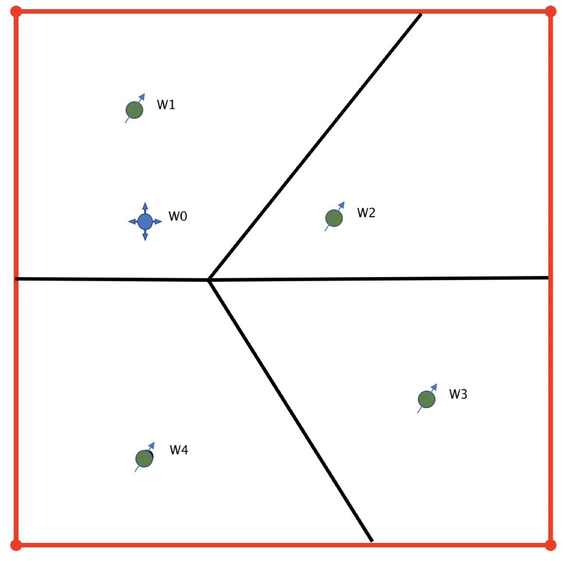
| Fig. 1. Location map of injector-producer pairing with 4 producers {W1, W2, W3, W4} and one injector W0. |
Case #1 – Constant flowrate production:
...
| q^{\uparrow}_1 = \rm const >0 |
|
The bottom-hole pressure response
in producer
W1 to the flowrate variation
| LaTeX Math Inline |
|---|
| body | \delta qq^{\downarrow}_0 |
|---|
|
in injector
W0:
| LaTeX Math Block |
|---|
|
\delta p_1 = - p_{u,\rm 21}(t) \cdot \delta qq^{\downarrow}_0 |
where
...
| Expand |
|---|
|
| Panel |
|---|
| borderColor | wheat |
|---|
| bgColor | mintcream |
|---|
| borderWidth | 7 |
|---|
| Consider a pressure convolution equation for the BHP in producer W1 with constant flowrate production at producer W1 | LaTeX Math Inline |
|---|
| body | qq^{\uparrow}_1 = \rm const |
|---|
|
and varying injection rate at injector W20 | LaTeX Math Inline |
|---|
| body | q_2q^{\downarrow}_0(t) |
|---|
|
:| LaTeX Math Block |
|---|
| p_1(t) = p_i - \int_0^t p_{u,\rm 11}(t-\tau) dqdq^{\uparrow}_1(\tau) - \int_0^t p_{u,\rm 01}(t-\tau) dqdq^{\downarrow}_0(\tau) = p_i - \int_0^t p_{u,\rm 01}(t-\tau) dqdq^{\downarrow}_0(\tau) |
Consider a step-change in injector's W0 flowrate | LaTeX Math Inline |
|---|
| body | \delta qq^{\downarrow}_0 |
|---|
|
at zero time , which can be writen as | LaTeX Math Block |
|---|
| q_0(\tau) = \delta qq^{\downarrow}_0 \cdot H(\tau) |
where is Heaviside step function:| LaTeX Math Block |
|---|
| H(\tau) = \begin{cases} 0, & \tau <0 \\ 1, &\tau \geq 0\end{cases} |
The differential then can be written as:| LaTeX Math Block |
|---|
| d qq^{\downarrow}_0(\tau) = q_0'(\tau) d\tau = \delta qq^{\downarrow}_0 \cdot H'(\tau) \, d\tau = \delta qq^{\downarrow}_0 \cdot \delta(\tau) \, d\tau |
The responding pressure variation in producer W1 will be:| LaTeX Math Block |
|---|
| \delta p_1(t) = p_1(t)-p_i = - \int_0^t p_{u,\rm 21}(t-\tau) \delta qq^{\downarrow}_0 \cdot \delta(\tau) \, d\tau = - p_{u,\rm 01}(t) \cdot \delta qq^{\downarrow}_0 |
which leads to | LaTeX Math Block Reference |
|---|
|
. |
|
...
Assume that the flowrate in producer W1 is being automatically adjusted by
| LaTeX Math Inline |
|---|
| body | \delta qq^{\uparrow}_1(t) |
|---|
|
to compensate the
bottom-hole pressure variation
in response to the
total sandface flowrate variation
| LaTeX Math Inline |
|---|
| body | \delta q_2q^{\downarrow}_0 |
|---|
|
in injector
W0 so that
bottom-hole pressure in producer
W1 stays constant at all times
| LaTeX Math Inline |
|---|
| body | \delta p_1(t) = \delta p_1 = \rm const |
|---|
|
. In petroleum practice this happens when the formation is capable to deliver more fluid than the current lift settings in producer so that the
bottom-hole pressure in producer is constantly kept at minimum value defined by the lift design..
In this case, flowrate response
| LaTeX Math Inline |
|---|
| body | \delta qq^{\uparrow}_1 |
|---|
|
in producer
W1 to the flowrate variation
| LaTeX Math Inline |
|---|
| body | \delta qq^{\downarrow}_0 |
|---|
|
in injector
W0 is going to be:
| LaTeX Math Block |
|---|
|
\delta qq^{\uparrow}_1(t) = - \frac^{\uparrow} \frac{\dot p_{u,\rm 01}(t)}{\dot p_{u,\rm 11}(t)} \cdot \delta qq^{\downarrow}_0 |
where
...
| Expand |
|---|
|
| Panel |
|---|
| borderColor | wheat |
|---|
| bgColor | mintcream |
|---|
| borderWidth | 7 |
|---|
| Consider a pressure convolution equation for the above 2-wells system with constant BHP: | LaTeX Math Block |
|---|
| p_1(t) = p_i - \int_0^t p_{u,\rm 11}(t-\tau) dqdq^{\uparrow}_1(\tau) - \int_0^t p_{u,\rm 01}(t-\tau) dqdq^{\downarrow}_0(\tau) = \rm const |
The time derivative is going to be zero as the BHP in producer W1 stays constant at all times: | LaTeX Math Block |
|---|
| \dot p_1(t) = - \left( \int_0^t p_{u,\rm 11}(t-\tau) dqdq^{\uparrow}_1(\tau) \right)^{\cdot} - \left( \int_0^t p_{u,\rm 01}(t-\tau) dqdq^{\downarrow}_0(\tau) \right)^{\cdot} = 0 |
| LaTeX Math Block |
|---|
| p_{u,\rm 11}(0) \cdot \dot qq^{\uparrow}_1(t) + \int_0^t \dot p_{u,\rm 11}(t-\tau) dqdq^{\uparrow}_1(\tau) = - p_{u,\rm 01}(0) \cdot \dot qq^{\downarrow}_0(t) - \int_0^t \dot p_{u,\rm 01}(t-\tau) dqdq^{\downarrow}_0(\tau) |
The zero-time value of DTR / CTR is zero by definition | LaTeX Math Inline |
|---|
| body | p_{u,\rm 11}(0) = 0, \, p_{u,\rm 01}(0) = 0 |
|---|
|
which leads to:| LaTeX Math Block |
|---|
| anchor | Case2_PSS_p11_temp |
|---|
| alignment | left |
|---|
| \int_0^t \dot p_{u,\rm 11}(t-\tau) dq_dq^{\uparrow}_1(\tau) = - \int_0^t \dot p_{u,\rm 2101}(t-\tau) dq_2dq^{\downarrow}_0(\tau) |
Consider a step-change in producer's W1 flowrate | LaTeX Math Inline |
|---|
| body | \delta qq^{\uparrow}_1 |
|---|
|
and injector's W0 flowrate | LaTeX Math Inline |
|---|
| body | \delta qq^{\downarrow}_0 |
|---|
|
at zero time , which can be written as | LaTeX Math Inline |
|---|
| body | dqdq^{\uparrow}_1(\tau) = \delta qq^{\uparrow}_1 \cdot \delta(\tau) \, d\tau |
|---|
|
.Assume that a lift mechanism in producer automatically adjusts the flowrate to maintain the same flowing bottom-hole and | LaTeX Math Inline |
|---|
| body | dqdq^{\downarrow}_0(\tau) = \delta qq^{\downarrow}_0 \cdot \delta(\tau) \, d\tau |
|---|
|
.Substituting this to | LaTeX Math Block Reference |
|---|
|
leads to:| LaTeX Math Block |
|---|
| \int_0^t \dot p_{u,\rm 11}(t-\tau) \delta qq^{\uparrow}_1 \cdot \delta(\tau) \, d\tau = - \int_0^t \dot p_{u,\rm 01}(t-\tau) \delta qq^{\downarrow}_0 \cdot \delta(\tau) \, d\tau |
| LaTeX Math Block |
|---|
| \dot p_{u,\rm 11}(t) \delta qq^{\uparrow}_1 = - \dot p_{u,\rm 01}(t) \delta qq^{\downarrow}_0 |
which leads to | LaTeX Math Block Reference |
|---|
|
. |
|
...
For the finite-volume drain
| LaTeX Math Inline |
|---|
| body | V_{\phi,1} \leq V_{\phi,0} < \infty |
|---|
|
the flowrate response factor
| LaTeX Math Inline |
|---|
| body | \delta qq^{\uparrow}_1 / \delta qq^{\downarrow}_0 |
|---|
|
is getting stabilised over time as:
| LaTeX Math Block |
|---|
| anchor | Case2_PSS |
|---|
| alignment | left |
|---|
|
\delta qq^{\uparrow}_1 / \delta qq^{\downarrow}_0 = - f_{01} = - \frac{V_{\phi, 1}}{ V_{\phi, 0}} = \rm const |
...
| LaTeX Math Block |
|---|
|
\delta qq^{\uparrow}_1 = -\delta qq^{\downarrow}_0 |
which means that producer W1 with constant BHP and finite-reservoir volume will eventually vary its rate at the same volume as injector W0.
...
| LaTeX Math Block |
|---|
|
\delta qq^{\uparrow}_1 =-\sum_i f_{i1} \delta qq^{\downarrow}_i
|
with constant coefficients | LaTeX Math Inline |
|---|
| body | f_{i1} \geq 0, \ {i=\{0..N_{\rm inj} \} } |
|---|
|
.
...
- Start with true UTRs
| LaTeX Math Inline |
|---|
| body | \displaystyle p_{u, ik}(t) |
|---|
|
with the same LTR asymptotic | LaTeX Math Inline |
|---|
| body | \displaystyle p_{u, ik}(t) \rightarrow \frac{t}{RS} |
|---|
|
. - Select injector W0
- Select producer W1
- Perform two a convolution tests to account for the impact from {W2 .. WN} production and from {W-1 .. W-M} on to DTRCTR_11 01 and CTR_01 :Test #1 – DTR_11Calculate interfering DTR_11:
| LaTeX Math Inline |
|---|
| body | \displaystyle p^*_{u, |
|---|
|
11 11k 1 k1| i1}(t) \cdot q^{\downarrow}_ |
|
k - Perform two convolution tests to account for the impact from {W2 .. WN} production on to DTR_11 , meaning that injector W0 is shut-down and all producers are working with constant rates
| q^*_k | , except producer W1 which is working with unit-rate Test #2 – and CTR_01 Calculate interfering CTR_01: \displaystyle p^*:- Test #1 – DTR_11
- Calculate interfering DTR_11:
| LaTeX Math Inline |
|---|
| body | \displaystyle p^*_{u, 11}(t) = = p_{u, 0111}(t) + \sum_{k \neq 1 \in {\rm prod}} p_{u, k1}(t) \cdot qq^{\uparrow}_k(t) |
|---|
|
, meaning that injector all injectors W0 is working with unit-rate are shut-down and all producers are were working with constant their historical rates , except producer W1 which is working with unit-rate
Calculate injection share constant- Test #2 – CTR_01
- Calculate interfering CTR_01:
f_{01} = \frac{\dot }{\dot p^*11} Bigg|t rightarrow \infty} as LLS over equation: | LaTeX Math Inline |
|---|
body | \displaystyle \dot p^*_{01| neq 0 \in {\rm inj}} p_{u, i1}(t) |
|
= f_{01} \dot p^*_{11}
- Repeat the same for other producers (starting from point 2a onwards)
Repeat the same for other injectors (starting from point 2 onwards)- , meaning that all producers are shut-down and all injectors are working with their historical rates , except injector W0 which is working with unit-rate
- Calculate injection share constant:
| LaTeX Math Inline |
|---|
| body | \displaystyle f_{01} = \frac{\dot p^*_{01}(t)}{\dot p^*_{11}(t)} \Bigg|_{t \rightarrow \infty} |
|---|
|
as LLS over equation: | LaTeX Math Inline |
|---|
| body | \displaystyle \dot p^*_{01}(t) = f_{01} \cdot \dot p^*_{11}(t) |
|---|
|
- Repeat the same for other producers (starting from point 2a onwards)
- Repeat the same for other injectors (starting from point 2 onwards)
| Show If |
|---|
|
| Expand |
|---|
|
| Panel |
|---|
| borderColor | wheat |
|---|
| bgColor | mintcream |
|---|
| borderWidth | 7 |
|---|
| Consider a pressure convolution equation for the well W1 with constant BHP in a multi-well system : | LaTeX Math Block |
|---|
| p_1(t) = p_i - \sum_{k \in {\rm prod}} \int_0^t p_{u,\rm k1}(t-\tau) dq^{\uparrow}_k(\tau) - \sum_{i \in {\rm inj}} \int_0^t p_{u,\rm i1}(t-\tau) dq^{\downarrow}_i(\tau) = \rm const |
The time derivative is going to be zero as the BHP in producer W1 stays constant at all times: | LaTeX Math Block |
|---|
| \dot p_1(t) = - \left( \sum_{k \in {\rm prod}} \int_0^t p_{u,\rm k1}(t-\tau) dq^{\uparrow}_k(\tau) \right)^\cdot -
\left( \sum_{i \in {\rm inj}} \int_0^t p_{u,\rm i1}(t-\tau) dq^{\downarrow}_i(\tau) \right)^\cdot = 0 |
| LaTeX Math Block |
|---|
| \sum_{k \in {\rm prod}} p_{u,\rm k1}(0) \dot q^{\uparrow}_k(t) +
\sum_{k \in {\rm prod}} \int_0^t \dot p_{u,\rm kk}(t-\tau) dq^{\uparrow}_k(\tau) =
- \sum_{i \in {\rm inj}} p_{u,\rm i1}(0) \dot q^{\downarrow}_i(t)
- \sum_{i \in {\rm inj}} \int_0^t \dot p_{u,\rm i1}(t-\tau) dq^{\downarrow}_i(\tau) |
The zero-time value of DTR / CTR is zero by definition | LaTeX Math Inline |
|---|
| body | p_{u,\rm kj}(0) = 0, \ \forall k,j \in \mathbb{Z} |
|---|
|
which leads to:| LaTeX Math Block |
|---|
| \sum_{k \in {\rm prod}} \int_0^t \dot p_{u,\rm k1}(t-\tau) dq^{\uparrow}_k(\tau) =
- \sum_{i \in {\rm inj}} \int_0^t \dot p_{u,\rm i1}(t-\tau) dq^{\downarrow}_i(\tau) |
Let's separate producer W1 and injector W0 terms: | LaTeX Math Block |
|---|
| anchor | pre_eq |
|---|
| alignment | left |
|---|
| \int_0^t \dot p_{u,\rm 11}(t-\tau) dq^{\uparrow}_1(\tau) + \sum_{k \neq 1 \in {\rm prod}} \int_0^t \dot p_{u,\rm k1}(t-\tau) dq^{\uparrow}_k(\tau) =
- \int_0^t \dot p_{u,\rm 01}(t-\tau) dq^{\downarrow}_0(\tau) - \sum_{i \neq 0 \in {\rm inj}} \int_0^t \dot p_{u,\rm i1}(t-\tau) dq^{\downarrow}_i(\tau) |
Consider a step-change in injector's W0 flowrate | LaTeX Math Inline |
|---|
| body | \delta q^{\downarrow}_0 |
|---|
|
at zero time , which can be written as | LaTeX Math Inline |
|---|
| body | dq^{\uparrow}_1(\tau) = \delta q^{\uparrow}_1 \cdot \delta(\tau) \, d\tau |
|---|
|
, leading to a step-change in production rate in producer W1| LaTeX Math Inline |
|---|
| body | dq^{\uparrow}_1(\tau) = \delta q^{\uparrow}_1 \cdot \delta(\tau) \, d\tau |
|---|
|
.Substituting this to | LaTeX Math Block Reference |
|---|
|
leads to:| LaTeX Math Block |
|---|
| \dot p_{u,\rm 11}(t) \delta q^{\uparrow}_1 + \sum_{k \neq 1 \in {\rm prod}} \int_0^t \dot p_{u,\rm k1}(t-\tau) dq^{\uparrow}_k(\tau) =
- \dot p_{u,\rm 01}(t) \delta q^{\downarrow}_0 - \sum_{i \neq 0 \in {\rm inj}} \int_0^t \dot p_{u,\rm i1}(t-\tau) dq^{\downarrow}_i(\tau) |
|
|
|
Again it is important to note a difference between
...