@wikipedia
A specific type of mathematical model of Decline Curve Analysis, based on the following equation:
| LaTeX Math Block |
|---|
|
q(t)=q_0 \cdot \left( 1+b \cdot D_0 \cdot t \right)^{-1/b} |
where
| Initial production rate of a well (or groups of wells) |
| initial Production decline rate (the higher the the stronger is decline) |
| defines the type of decline (see below) |
It can be applied to any fluid production: water, oil or gas.
The cumulative production is then given by:
| LaTeX Math Block |
|---|
|
Q(t)=\int_0^t q(t) \, dt |
The Production Decline Rate is given by:
| LaTeX Math Block |
|---|
|
D(t) = - \frac{dq}{dQ} = \frac{D_0}{1+ b \cdot D_0 \cdot t} |
The ultimate recovery is defined as:
| LaTeX Math Block |
|---|
|
Q_{\rm max}=Q(t=\infty)=\int_0^\infty q(t) \, dt =\frac{q_0}{D_0 \cdot (1-b)} |
Arp's model splits into three types based on the value of
coefficient:
| Exponential Production Decline | Hyperbolic Production Decline | Harmonic Production Decline |
|---|
| | |
| LaTeX Math Block |
|---|
| q(t)=q_0 \exp \left( -D_0 \, t \right) |
|
| LaTeX Math Block |
|---|
| q(t) = \frac{q_0}{ \left( 1+b \cdot D_0 \cdot t \right)^{1/b} } |
|
| LaTeX Math Block |
|---|
| q(t)=\frac{q_0}{1+D_0 \, t} |
|
| LaTeX Math Block |
|---|
| Q(t)=\frac{q_0-q(t)}{D_0} |
|
| LaTeX Math Block |
|---|
| Q(t)=\frac{q_0}{D_0 \, (1-b)} \, \left[ 1- \left( \frac{q(t)}{q_0} \right)^{1-b} \right]
|
|
| LaTeX Math Block |
|---|
| Q(t)=\frac{q_0}{D_0} \, \ln \left[ \frac{q_0}{q(t)} \right] |
|
| LaTeX Math Block |
|---|
| D(t) = D_0 = \rm const |
|
| LaTeX Math Block |
|---|
| D(t) =\frac{D_0}{1+ b \cdot D_0 \cdot t} |
|
| LaTeX Math Block |
|---|
| D(t) = \frac{D_0}{1+ D_0 \cdot t} |
|
| LaTeX Math Block |
|---|
| Q_{\rm max}=\frac{q_0}{D_0} |
|
| LaTeX Math Block |
|---|
| Q_{\rm max}=\frac{q_0}{D_0 \cdot (1-b)} |
|
| LaTeX Math Block |
|---|
| Q_{\rm max}=\infty |
|
The Exponential and Hyperbolic decline are applicable for Boundary Dominated Flow with finite reserves
| LaTeX Math Inline |
|---|
| body | --uriencoded--Q_%7B\rm max%7D \leq \infty |
|---|
|
while
Harmonic decline is associated with production from the reservoir with infinite reserves
| LaTeX Math Inline |
|---|
| body | --uriencoded--Q_%7B\rm max%7D = \infty |
|---|
|
. In other words the
Harmonic decline is very slow.
Since all physical reserves are finite the true meaning of Harmonic decline is that up to date it did not reach the boundary of these reserves and at certain point in future it will transform into a finite-reserves decline (possibly Exponential or Hyperbolic).
Exponential Production Decline has a physical meaning of declining production from finite drainage volume
with constant
BHP:
| LaTeX Math Inline |
|---|
| body | p_{wf}(t) = \rm const |
|---|
|
(a specific type of
Boundary Dominated Flow under
Pseudo Steady State (PSS) conditions).
Harmonic and Hyperbolic declines are both empirical.
The DCA Arps do not cover all types of production decline, but their application is quite broad and mathematics is quite simple which gained popularity as quick estimation of production perspectives.
See Also
Petroleum Industry / Upstream / Production / Subsurface Production / Field Study & Modelling / Production Analysis / Decline Curve Analysis
[ Exponential Production Decline ][ Hyperbolic Production Decline ][ Harmonic Production Decline ]
[ Production Decline Rate ]
References
Arps, J. J. (1945, December 1). Analysis of Decline Curves. Society of Petroleum Engineers. doi:10.2118/945228-G
| Show If |
|---|
|
| Panel |
|---|
|
| Expand |
|---|
|
Введение
Экспресс-Анализ Кривых Падения Дебитов (DCA = Decline Curve Analysis) ставит своей задачей оценить будущую динамику добычи скважины (или группы скважин) на основе известной предыстории.
Традиционные методы анализа (типа Арпс) основаны на эмпирических формулах и используют для анализа только информацию о дебитах скважин.
Современные методы, помимо данных о дебитах, вовлекают в анализ имеющуюся информацию о давлении и моделируют поведение кривых на основе решения уравнения диффузии давления в пласте, что часто побуждает относить эти методы к разделу ГДИ. Математические модели
Метод Арпс (Arps) является исторически первым и до сих пор одним из самых популярных на практике методом предсказания динамики добычи без привлечения сведений о давлении в пластах.
В основе метода лежит следующая эмпирическая формула для дебита: | LaTeX Math Block |
|---|
| q(t)=\frac{q_{i}}{[1+b \, D \, t]^{\frac{1}{b}}} |
Коэффициент имеет смысл начального дебита скважины (или группы скважин),а коэффициент | LaTeX Math Block |
|---|
| D=-\frac{1}{q}\frac{dq}{dt} |
имеет смысл декремента падения добычи (чем больше тем сильнее будет падать добыча со временем).
Для анализа также используется накопленная добыча: | LaTeX Math Block |
|---|
| Q(t)=\int_0^t q(t) dt |
На практике различают четыре разновидности Арпс-режимов:
|
|
|
|---|
| Экспоненциальный | b = 1 |
| LaTeX Math Block |
|---|
| q(t)=q_{i} \exp \big [ -D \, t \big ] |
| LaTeX Math Block |
|---|
| Q(t)=\frac{q_{i}-q(t)}{D} |
| | Гармонический | b = 0 |
| LaTeX Math Block |
|---|
| q(t)=\frac{q_{i}}{[1+D \, t]} |
| LaTeX Math Block |
|---|
| Q(t)=\frac{q_{i}}{D}\ln (\frac{q_{i}}{q(t)}) |
| | Гиперболический | b = 0..1 |
| LaTeX Math Block |
|---|
| q(t)=\frac{q_{i}}{[1+b \, D \, t]^{\frac{1}{b}}} |
| LaTeX Math Block |
|---|
| Q(t)=\frac{q_{i}}{D \, (1-b)}(q_{i}^{1-b}-q(t)^{1-b})
|
| | Power Loss |
| LaTeX Math Block |
|---|
| D=D_{\infty} + \frac{t^{n-1}}{\tau^{n}} |
|
| LaTeX Math Block |
|---|
| q(t)=q_{i} \exp \big [ -D_{\infty}t- \bigg(\frac{t}{\tau} \bigg)^{n} \big] |
|
Хотя в целом такой подход является феноменологическим, конкретно экспоненциальный режим падения добычи имеет физическое обоснование, представляя собой режим псевдо-стационарной радиальной фильтрации в замкнутом резервуаре.
Результат работы солвера: 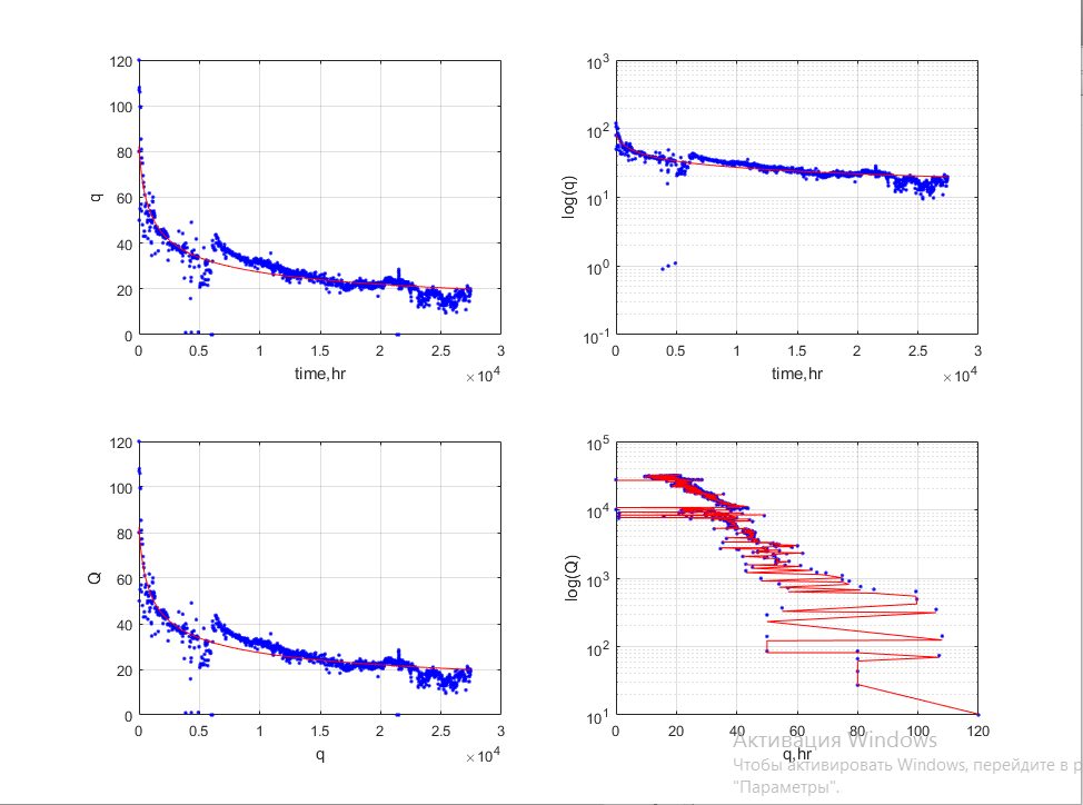
Графические представления
Просматривать график лучше используя коэф-т потерь Арпса: 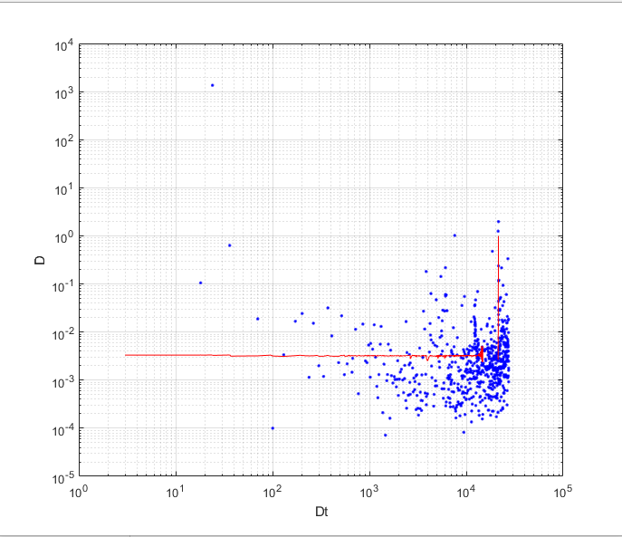
|
|
|