...
|
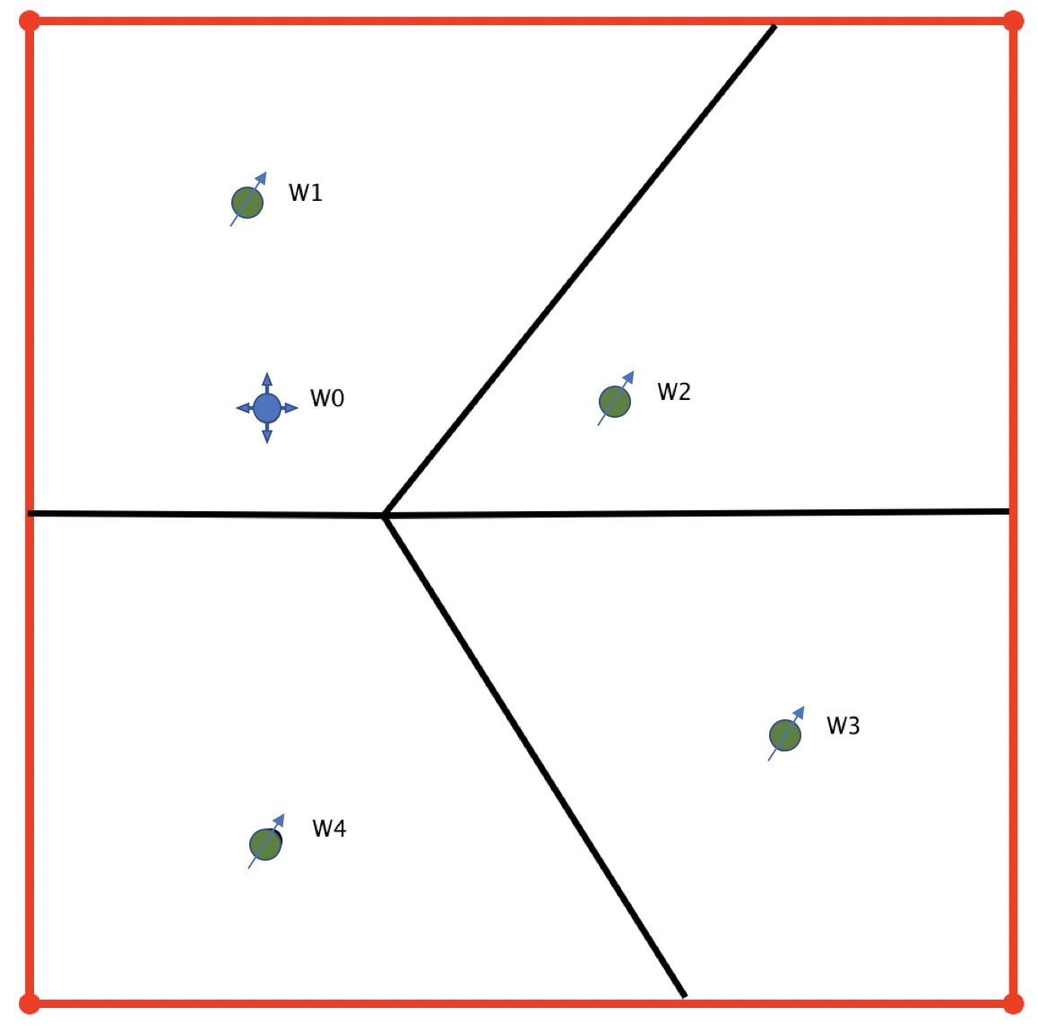
| Fig. 1. Location map of injector-producer pairing with 4 producers {W1, W2, W3, W4} and one injector W0. |
Case #1 – Constant flowrate production:
The bottom-hole pressure response
in producer
W1 to the flowrate variation
in injector
W0:
...
| Expand |
|---|
|
| Panel |
|---|
| borderColor | wheat |
|---|
| bgColor | mintcream |
|---|
| borderWidth | 7 |
|---|
| Consider a pressure convolution equation for the BHP in producer W1 with constant flowrate production at producer W1 and varying injection rate at injector W2 :| LaTeX Math Block |
|---|
| p_1(t) = p_i - \int_0^t p_{u,\rm 11}(t-\tau) dq_1(\tau) - \int_0^t p_{u,\rm 01}(t-\tau) dq_0(\tau) = p_i - \int_0^t p_{u,\rm 01}(t-\tau) dq_0(\tau) |
Consider a step-change in injector's W0 flowrate at zero time , which can be written as: | LaTeX Math Inline |
|---|
| body | dq_0 (\tau) = \delta q_0 \cdot \delta(\tau) \, d\tau |
|---|
|
.The responding pressure variation in producer W1 will be:| LaTeX Math Block |
|---|
| \delta p_1(t) = p_1(t)-p_i = - \int_0^t p_{u,\rm 21}(t-\tau) \delta q_0 \cdot \delta(\tau) \, d\tau = - p_{u,\rm 01}(t) \cdot \delta q_0 |
which leads to | LaTeX Math Block Reference |
|---|
|
. |
|
Case #2 – Constant BHP:
Assume that the flowrate in producer W1 is being automatically adjusted by
to compensate the
bottom-hole pressure variation
in response to the
total sandface flowrate variation
in injector
W0 so that
bottom-hole pressure in producer
W1 stays constant at all times
| LaTeX Math Inline |
|---|
| body | \delta p_1(t) = \delta p_1 = \rm const |
|---|
|
. In petroleum practice this happens when the formation is capable to deliver more fluid than the current lift settings in producer so that the
bottom-hole pressure in producer is constantly kept at minimum value defined by the lift design..
...
| Expand |
|---|
|
| Panel |
|---|
| borderColor | wheat |
|---|
| bgColor | mintcream |
|---|
| borderWidth | 7 |
|---|
| For the finite-volume reservoir | LaTeX Math Inline |
|---|
| body | V_{\phi,1} \leq V_{\phi,0} < \infty |
|---|
|
the DTR and CTR are both going through the PSS flow regime at late transient times:
| LaTeX Math Block |
|---|
| anchor | Case2_PSS_p11 |
|---|
| alignment | left |
|---|
| p_{u,\rm 11}(t \rightarrow \infty) \rightarrow \frac{t}{c_t V_{\phi, 1}} |
|
| LaTeX Math Block |
|---|
| anchor | Case2_PSS_p21 |
|---|
| alignment | left |
|---|
| p_{u,\rm 01}(t \rightarrow \infty) \rightarrow \frac{t}{c_t V_{\phi,2}} |
|
where Substituting | LaTeX Math Block Reference |
|---|
|
and | LaTeX Math Block Reference |
|---|
|
in | LaTeX Math Block Reference |
|---|
|
one arrives to | LaTeX Math Block Reference |
|---|
|
. |
|
...
| LaTeX Math Block |
|---|
|
\sum_{k=1}^N f_{0k} = 1 |
with constant coefficients | LaTeX Math Inline |
|---|
| body | f_{0k} \geq 0, \ {k=\{i..N \} } |
|---|
|
, unless there is a thief injection outside the drain drainage area of all producers and in this case:
| LaTeX Math Block |
|---|
| anchor | fokless1 |
|---|
| alignment | left |
|---|
|
\sum_{k=1}^N f_{0k} < 1 |
If pressure in producer around producer W1 is supported by several injectors
then
over a long period of time one can assume:
| LaTeX Math Block |
|---|
|
\delta q_1 =\sum_k f_{k1i1} \delta q_ki
|
with constant coefficients | LaTeX Math Inline |
|---|
| body | f_{1ki1} \geq 0, \ {k=\{1i..N_{\rm inj} \} } |
|---|
|
.
The equations | LaTeX Math Block Reference |
|---|
|
, | LaTeX Math Block Reference |
|---|
|
and | LaTeX Math Block Reference |
|---|
|
make one of the key assumptions in Capacitance Resistance Model (CRM).
It is important to note that assumption that injector W0 may drain bigger volume than producer W1 | LaTeX Math Inline |
|---|
| body | V_{\phi, 0}> V_{\phi, 1} |
|---|
|
is a misnomer.
When wells (producers and injectors) are placed into interconnected reservoir volume they drain the same volume alltogether and the DTR/CTR will have the same LTR asymptotic:
| LaTeX Math Block |
|---|
|
p_{u,\rm ik}(t \rightarrow \infty ) \rightarrow \frac{t}{c_t \, V_\phi}, \forall i,k. |
Moreover, if each well is placed in different reservoir volumes which are only connected through wellbores then again they will all drain the same volume which is the sum of all connected volumes through the wellbores and the DTR/CTR will again trend to the same LTR asymptotic.
In order to relate the DTR/CTR from numerical grid simulations or from deconvolution theory to the CRM injection share constants one need to implement a following trick.
See also
...
[ DTR ] [ CTR ] [ Capacitance Resistance Model (CRM) ]
...