Single-well Pressure Pulsation survey

Motivation

One of the most important objectives of the well testing is to assess the drainable hydrocarbon reserves and reservoir properties around tested well.

This particularly becomes important in appraisal drilling as well testing is the only source of this information.

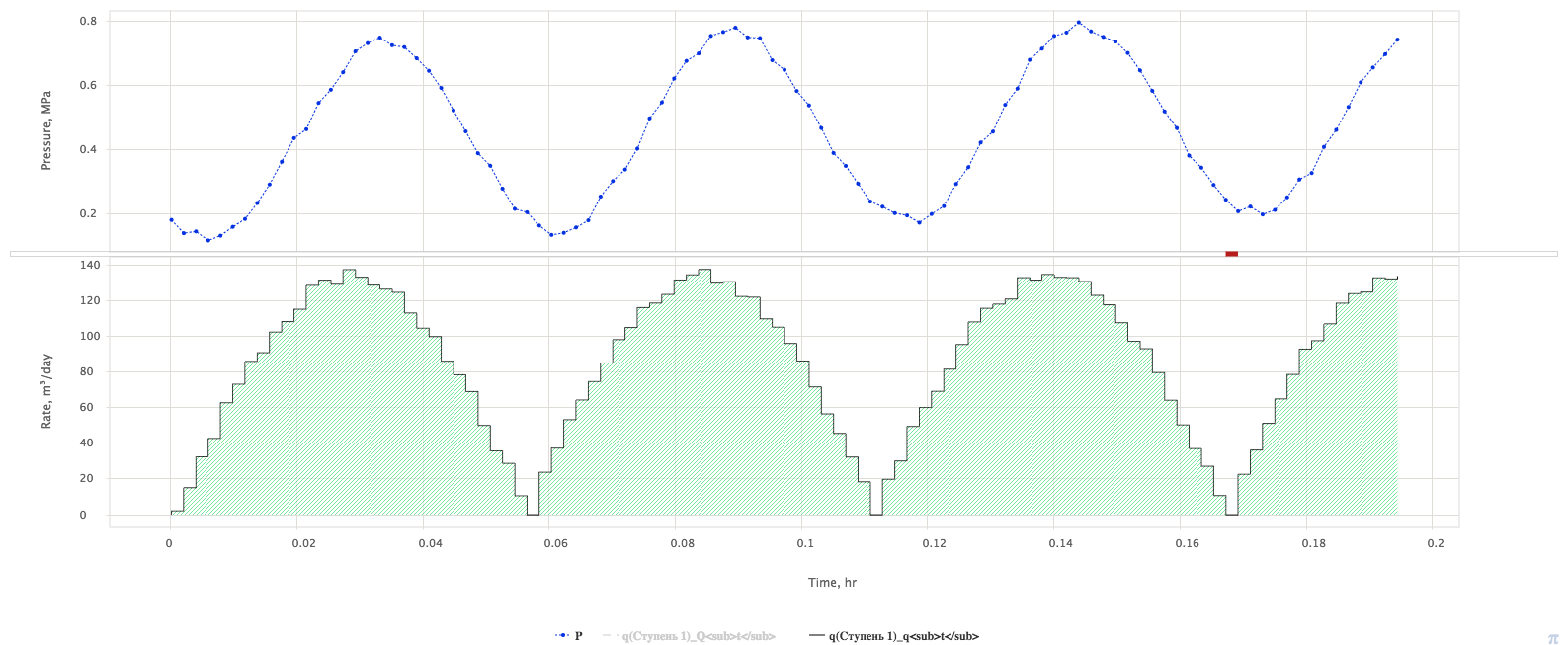
The Self-Pulse Test (SPT) is a single-well pressure test with periodic changes in flow rate and pressure (see Fig. 1).

Fig. 1. Typical record of pressure and rate variation during SPT

Expand on analytical approach

When flow rate is being intentionally varied in harmonic cycles with sandface amplitude $\begin{array}{l}q_0\end{array}$ and cycling frequency $\begin{array}{l}\omega = \frac{2 \, \pi}{T}\end{array}$ :

(1)	$\begin{array}{l}\displaystyle q(t) = q_0 \, \sin ( \omega \, t )\end{array}$

then bottom-hole pressure will follow the same variation pattern:

(2)	$\begin{array}{l}\displaystyle p_{wf}(t) = p_0 \, \sin ( \omega \, [ t - t_{\Delta} ] )\end{array}$

with a bottom-hole pressure amplitude $\begin{array}{l}p_0\end{array}$ and the time delay $\begin{array}{l}t_{\Delta}\end{array}$ .

It takes some time (3-5 cycles $\begin{array}{l}t \geq 3 \, T\end{array}$ ) for pressure to develop a stabilized response to rate variations.

The pressure delay $\begin{array}{l}t_{\Delta}\end{array}$ and associated dimensionless phase shift $\begin{array}{l}\Delta = \omega \, t_{\Delta}\end{array}$ represent the inertia effects from the adjoined reservoir and characterized by formation pressure diffusivity:

(3)	$\begin{array}{l}\displaystyle \chi = \Big < \frac{k}{\mu} \Big > \frac{1}{\phi \, c_t}\end{array}$

The diffusion nature of pressure dictates that amplitude of pressure variation is proportional to amplitude of sandface flowerate variation and the ratio $\begin{array}{l}\frac{p_0}{q_0}\end{array}$ is related to formation transmissibility:

(4)	$\begin{array}{l}\displaystyle \sigma = \Big < \frac{k}{\mu} \Big > \, h\end{array}$

The exact solution of differential diffusion equation for vertical well with negligible well storage and infinite boundary homogeneous reservoir can be represented by a system of non-linear algebraic equations, relating field-measured parameters $\begin{array}{l}\big\{ \frac{q_0}{p_0}, \, t_{\Delta} \big\}\end{array}$ to formation properties $\begin{array}{l}\{ \sigma, \, \chi \}\end{array}$ :

(5)	$\begin{array}{l}\displaystyle X =r_w \, \sqrt{ \frac{\omega}{\chi} }\end{array}$

(6)	$\begin{array}{l}\displaystyle \Delta = \omega \, t_{\Delta} = \frac{\pi}{4} - arctg{ \frac{Ker_1 X \cdot Kei \, X - Ker_1 X \cdot Kei \, X }{Ker_1 X \cdot Kei \, X +Ker_1 X \cdot Kei \, X } }\end{array}$

(7)	$\begin{array}{l}\displaystyle \sigma =\frac{1}{2 \pi} \, \frac{q_0}{p_0} \, \sqrt{ \frac{Ker^2 X + Kei^2 X}{Ker_1^2 X + Kei_1^2 X} }\end{array}$

The above equations assume that diffusivity $\begin{array}{l}\chi\end{array}$ and dimensionless radius $\begin{array}{l}X\end{array}$ are found from (5) – (6) and then $\begin{array}{l}X\end{array}$ is substituted to (7) to calculate transmissibility $\begin{array}{l}\sigma\end{array}$ .

In case of a low frequency pulsations:

(8)	$\begin{array}{l}\displaystyle \omega \ll 0.00225 \, \frac{ \chi }{ r_w^2} \quad \Longleftrightarrow \quad X \ll 0.15\end{array}$

the equations (5) – (7) can be explicitly resolved in terms of transmissibility and diffusivity:

(9)	$\begin{array}{l}\displaystyle \chi = 0.25 \, \omega \, \gamma^2 \, r_w^2 \, \exp \frac{\pi}{2 \, {\rm tg} \Delta }\end{array}$

(10)	$\begin{array}{l}\displaystyle \sigma = \frac{q_0}{8 \, p_0 \, \sin \Delta}\end{array}$

where $\begin{array}{l}\Delta = \omega \, t_{\Delta}\end{array}$ .

The above analytical approach (either (5) – (7) or (9) – (10)) is rarely helpful in practise.

The field operations are very finnicky and difficult to follow the pre-desgined sequence of clean harmonic pulsations.

As result, the flowrate variation becomes a complex sum of harmonics:

(11)	$\begin{array}{l}\displaystyle q(t) = q_0 + \sum_{n=0}^\infty q_n \, \sin ( \omega_n \, t )\end{array}$

and the pressure response becomes complex as well:

(12)	$\begin{array}{l}\displaystyle p_{wf}(t) = p_0 + \sum_{n=0}^\infty p_n \, \sin ( \omega_n \, [ t - t_{\Delta_n} ] )\end{array}$

The use of analytical formulas requires fourier transformation to identify the key harmonics from the raw data with a manual control from analyst and a certain amount of subjectivism on which harmonics to pick up for calculating the transmissibility and diffusivity.

Once the harmonics are identified one need to search for the $\begin{array}{l}\{ \sigma, \, \chi \}\end{array}$ best fit to a complex system of non-linear algebraic equations:

(13)	$\begin{array}{l}\displaystyle X_n =r_w \, \sqrt{ \frac{\omega_n}{\chi} }\end{array}$

(14)	$\begin{array}{l}\displaystyle \Delta_n = \omega_n \, t_{\Delta} = \frac{\pi}{4} - arctg{ \frac{Ker_1 X_n \cdot Kei \, X_n - Ker_1 X_n \cdot Kei \, X_n }{Ker_1 X_n \cdot Kei \, X_n +Ker_1 X_n \cdot Kei \, X_n } }\end{array}$

(15)	$\begin{array}{l}\displaystyle \sigma =\frac{1}{2 \pi} \, \frac{q_n}{p_n} \, \sqrt{ \frac{Ker^2 X_n + Kei^2 X_n}{Ker_1^2 X_n + Kei_1^2 X_n} }\end{array}$

In practice, the most efficient methodology to interpret the SPT data is via fitting numerical model to the raw pressure-rate data.

Still, formulas (9) and (10) play important academic role and provide fast track estimations in SPT engineering.

Expand more on the pressure-rate time lag in SPT

The effect of the pressure response delay $\begin{array}{l}\Delta\end{array}$ to flow rate variation in a single well test is so small (usually seconds) that conventional build-up can not capture it reliably due to a high pressure contamination and wellbore instability at early build-up times and hence pressure diffusivity normally can not be assessed.

In SPT the rate undergoes sequential step changes which allows data stacking and more accurate measurement of pressure-rate time lag and through this assess pressure diffusivity.

This effect is accurately described by analytical solution of diffusivity equation and meets practical observations.

In order to numerically reproduce a short-term pressure-rate time lag in single-well survey one needs a dedicated numerical solver since the required mesh size is very small and comparable to the well size and conventional Peaceman well model does not work (see also Numerical solutions for single-phase pressure diffusion @model).

Objectives

Assess reservoir volume around well
Assess reservoir permeability and thickness variation around well

Deliverables

The advantages of SPT deliverables over conventional single-well test is illustrated below.


V_hc	Potential hydrocarbon reserves
V_e	Drainage volume
A_e	Drainage area
k_near	Permeability of the near-reservoir zone
h_near	Effective thickness of the near-reservoir zone
k_far	Permeability of the far-reservoir zone
h_far	Effective thickness of the far-reservoir zone
S	Skin-factor
P_u(t)	Deconvolution of the long-term unit-rate response

Inputs

Property	Description	Data Source
B_o	Oil Formation Volume Factor	PVT samples / Correlations
Bg	Gas Formation Volume Factor	PVT samples / Correlations
B_w	Water Formation Volume Factor	PVT samples / Correlations
c_o	Oil compressibility	PVT samples / Correlations
c_w	Water compressibility	PVT samples / Correlations
cg	Gas compressibility	PVT samples / Correlations
c_r	Rock compressibility	Core samples / Correlations
s_wi	Initial water saturation	Core samples
$\begin{array}{l}\phi\end{array}$	Porosity	Core samples

Procedure

The typical SPT procedure is brought on Fig. 2.

Fig. 2. Typical SPT procedure

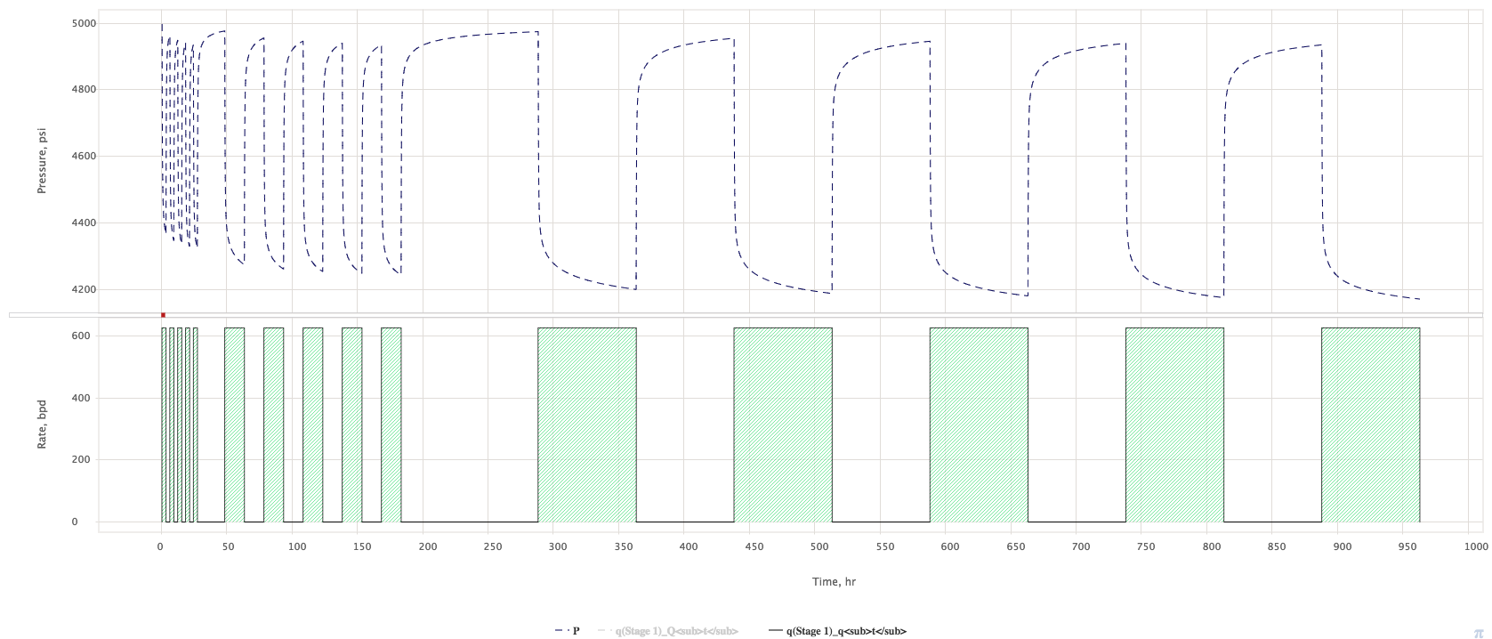
It normally consists ion three consequent tests with three different cycling frequencies:

Test 1 = high freq pulsations (5 pulses with period T)
Test 2 = mid freq pulsations (5 pulses with with period 5T)
Test 3 = Low freq pulsations (5 pulses with period 25 T)

The total duration of the test is 155 T.

Typically T = 3 hrs and total test duration is around 20 days.

Every pulse includes one choke-up and one choke-down so that full SPT survey require 60 choke operations during 40 days which is a lot of field activity for a given well.

It would be extremely difficult to perform this manually and usual practice is to arrange a programmable remote-controlled flow variation.

Model

SPT Model

Interpretation

Automated flowrate-pressure fata records match in multiphase 2D pressure simulator with:

Single well and circle boundary
High density LGR (meters)
High density time grid (seconds)

Page tree

Motivation

Deliverables

Inputs

Procedure

Model

Interpretation

See Also

References

Page tree

Self-Pulse Test (SPT) @survey

Motivation

Deliverables

Inputs

Procedure

Model

Interpretation

See Also

References