Consider a system of net hydrocarbon pay and finite volume Aquifer as a radial composite reservoir with inner composite area being a Net Pay Area and outer composite area an Aquifer

(see schematic and notations on Fig. 1 at Radial VEH Aquifer Drive @model).

The Aquifer's outer boundary may be "no-flow" or full pressure support, thus implementing the case of the infinite-volume Aquifer.

The transient pressure diffusion in the outer (Aquifer) composite area is going to honour the following equation:

(1)	$\begin{array}{l}\displaystyle \frac{\partial p_a}{\partial t} = \chi \cdot \left[ \frac{\partial^2 p_a}{\partial r^2} + \frac{1}{r}\cdot \frac{\partial p_a}{\partial r} \right]\end{array}$

(2)	$\begin{array}{l}\displaystyle p_a(t = 0, r)= p(0)\end{array}$

(3)	$\begin{array}{l}\displaystyle p_a(t, r=r_e) = p(t)\end{array}$

(4)	$\begin{array}{l}\displaystyle \frac{\partial p_a}{\partial r} \bigg\|_{(t, r=r_a)} = 0\end{array}$

or

(5)	$\begin{array}{l}\displaystyle p_a(t, r = \infty) = 0\end{array}$

Consider dimensionless solution $\begin{array}{l}p_1(t_D, r_D)\end{array}$ of the following equation:

(6)	$\begin{array}{l}\displaystyle \frac{\partial p_1}{\partial t_D} = \frac{\partial^2 p_1}{\partial r_D^2} + \frac{1}{r_D}\cdot \frac{\partial p_1}{\partial r_D}\end{array}$

(7)	$\begin{array}{l}\displaystyle p_1(t_D = 0, r_D)= 0\end{array}$

(8)	$\begin{array}{l}\displaystyle p_1(t_D, r_D=1) = 1\end{array}$

(9)	$\begin{array}{l}\displaystyle \frac{\partial p_1(t_D, r_D)}{\partial r_D} \Bigg\|_{r_D=r_{aD}} = 0\end{array}$

or

(10)	$\begin{array}{l}\displaystyle p_1(t_D, r_D = \infty) = 0\end{array}$

which represents a specific function of dimensionless time $\begin{array}{l}t_D\end{array}$ and distance $\begin{array}{l}r_D\end{array}$ .

Now consider a convolution integral:

(11)	$\begin{array}{l}\displaystyle p_a(t, r) = p(0) + \int_0^t p_1 \left(\frac{(t-\tau) \cdot \chi}{r_e^2}, \frac{r}{r_e} \right) \dot p(\tau) d\tau\end{array}$

(12)	$\begin{array}{l}\displaystyle \dot p(\tau) = \frac{d p}{d \tau}\end{array}$

One can easily check that (11) honours the whole set of equations (1)– (4) and as such defines a unique solution of the above problem.

Water flowrate within $\begin{array}{l}\theta\end{array}$ sector angle at interface with oil reservoir will be:

(13)	$\begin{array}{l}\displaystyle q^{\downarrow}_{AQ}(t)= \theta \cdot r_e \cdot h \cdot u(t,r_e)\end{array}$

where $\begin{array}{l}u(t,r_e)\end{array}$ is flow velocity at aquifer contact boundary, which is:

(14)	$\begin{array}{l}\displaystyle u(t,r_e) = M \cdot \frac{\partial p_a(t,r)}{\partial r} \bigg\|_{r=r_e}\end{array}$

where $\begin{array}{l}\displaystyle M = \frac{k_w}{\mu_w}\end{array}$ is aquifer mobility.

Water flowrate becomes:

(15)	$\begin{array}{l}\displaystyle q^{\downarrow}_{AQ}(t)= \theta \cdot r_e \cdot h \cdot M \cdot \frac{\partial p_a(t,r)}{\partial r} \bigg\|_{r=r_e}\end{array}$

Cumulative water flux:

(16)	$\begin{array}{l}\displaystyle Q^{\downarrow}_{AQ}(t) = \int_0^t q^{\downarrow}_{AQ}(t) dt = \theta \cdot r_e \cdot h \cdot M \cdot \int_0^t \frac{\partial p_a(t,r)}{\partial r} \bigg\|_{r=r_e} dt\end{array}$

Substituting (11) into (16) leads to:

(17)	$\begin{array}{l}\displaystyle Q^{\downarrow}_{AQ}(t) = \theta \cdot r_e \cdot h \cdot M \cdot \int_0^t d\xi \ \frac{\partial }{\partial r} \left[ \int_0^\xi p_1 \left( \frac{(\xi-\tau)\chi}{r_e^2}, \frac{r}{r_e} \right) \, \dot p(\tau) d\tau \right]_{r=r_e}\end{array}$

(18)	$\begin{array}{l}\displaystyle Q^{\downarrow}_{AQ}(t) = \theta \cdot h \cdot M \cdot \int_0^t d\xi \ \frac{\partial }{\partial r_D} \left[ \int_0^\xi p_1 \left( \frac{(\xi-\tau)\chi}{r_e^2}, r_D \right) \, \dot p(\tau) d\tau \right]_{r_D=1}\end{array}$

(19)	$\begin{array}{l}\displaystyle Q^{\downarrow}_{AQ}(t) = \theta \cdot h \cdot M \cdot \int_0^t d\xi \ \int_0^\xi \frac{\partial p_1}{\partial r_D} \left( \frac{(\xi-\tau)\chi}{r_e^2}, r_D \right) \Bigg\|_{r_D=1} \, \dot p(\tau) d\tau\end{array}$

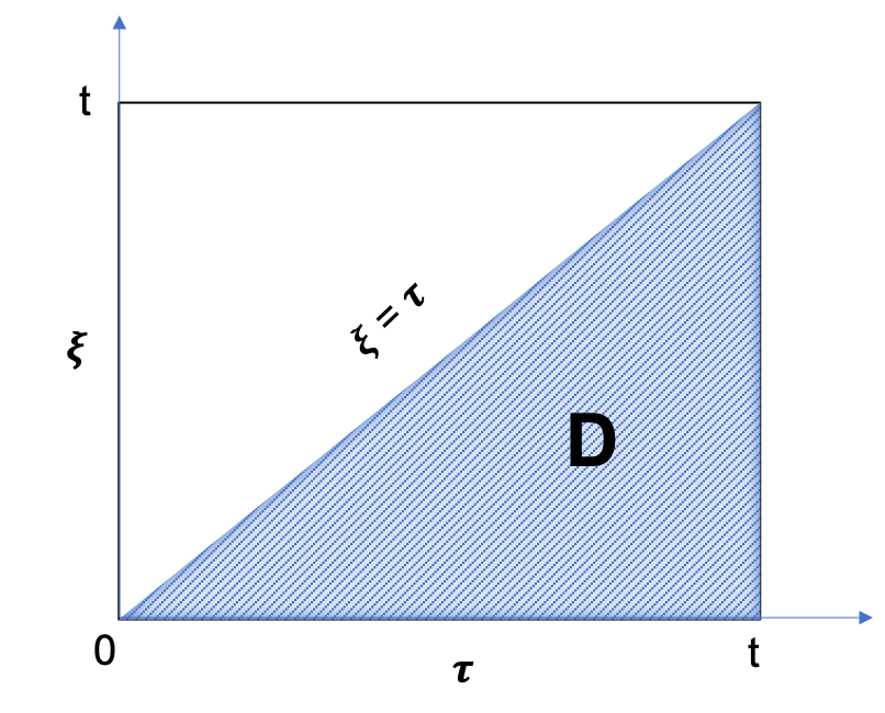
The above integral represents the integration over the $\begin{array}{l}D\end{array}$ area in $\begin{array}{l}(\tau, \ \xi)\end{array}$ plane (see Fig. 1):

(20)	$\begin{array}{l}\displaystyle Q^{\downarrow}_{AQ}(t) = \theta \cdot h \cdot M \cdot \iint_D d\xi \ d\tau \, \dot p(\tau) \frac{\partial p_1}{\partial r_D} \left( \frac{(\xi-\tau)\chi}{r_e^2}, r_D \right) \Bigg\|_{r_D=1}\end{array}$

Fig. 1. Illustration of the integration $\begin{array}{l}D\end{array}$ area in $\begin{array}{l}(\tau, \ \xi)\end{array}$ plane

Changing the integration order from $\begin{array}{l}\tau \rightarrow \xi\end{array}$ to $\begin{array}{l}\xi \rightarrow \tau\end{array}$ leads to:

(21)

$\begin{array}{l}\displaystyle Q^{\downarrow}_{AQ}(t) = \theta \cdot h \cdot M \cdot \int_0^t d\tau \int_\tau^t d\xi \ \dot p(\tau) \frac{\partial p_1}{\partial r_D} \left( \frac{(\xi-\tau)\chi}{r_e^2}, r_D \right) \Bigg|_{r_D=1} = \theta \cdot h \cdot M \cdot \int_0^t \dot p(\tau) d\tau \int_\tau^t d\xi \ \frac{\partial p_1}{\partial r_D} \left( \frac{(\xi-\tau)\chi}{r_e^2}, r_D \right) \Bigg|_{r_D=1}\end{array}$

Replacing the variable:

(22)	$\begin{array}{l}\displaystyle \xi = \tau + \frac{r_e^2}{\chi} \cdot t_D \rightarrow t_D = \frac{(\xi-\tau)\chi}{r_e^2} \rightarrow d\xi = \frac{r_e^2}{\chi} \cdot dt_D\end{array}$

and flux becomes:

(23)

$\begin{array}{l}\displaystyle Q^{\downarrow}_{AQ}(t) = \theta \cdot h \cdot M \cdot \frac{r_e^2}{\chi} \cdot \int_0^t \dot p(\tau) d\tau \int_0^{(t-\tau)\chi/r_e^2} \frac{\partial p_1( t_D, r_D)}{\partial r_D} \Bigg|_{r_D=1} dt_D = B \cdot \int_0^t \dot p(\tau) d\tau \int_0^{(t-\tau)\chi/r_e^2} \frac{\partial p_1( t_D, r_D)}{\partial r_D} \Bigg|_{r_D=1} dt_D\end{array}$

where $\begin{array}{l}B\end{array}$ is water influx constant and which leads to

Error rendering macro 'mathblock-ref' : Math Block with anchor=VEH could not be found.

and

Error rendering macro 'mathblock-ref' : Math Block with anchor=WeD could not be found.

.

Page tree

See Also

Page tree

Derivation of Radial VEH Aquifer Drive @model

See Also