Content

Definition

Mathematical model of multiphase wellbore flow predicts the temperature, pressure and flow speed distribution along the wellbore trajectory with account for:

tubing head pressure which is set by gathering system or injection pump
wellbore design
pump characterisits
fluid friction with tubing /casing walls
interfacial phase slippage
heat exchange between wellbore fluid and surrounding rocks

The $\begin{array}{l}\alpha\end{array}$ -phase flow fraction ( also called phase cut or input hold-up or no-slip hold-up ) is defined as:

(1)	$\begin{array}{l}\displaystyle \gamma_\alpha = \frac{q_\alpha}{q_t}\end{array}$

where $\begin{array}{l}q_\alpha\end{array}$ – volumetric flow rate of $\begin{array}{l}\alpha\end{array}$ -phase and $\begin{array}{l}q_t\end{array}$ is the total volumetric fluid production rate:

(2)	$\begin{array}{l}\displaystyle q_t = \sum_\alpha q_\alpha\end{array}$

The multiphase wellbore flow assumes that every phase occupies its own area of the total cross-sectional area of the lifting pipe.

This area can be connected into a single piece of cross-sectional area (like in case of annular flow) or disconnected into a number of spots (like in case of bubbly flow).

A share of total pipe cross-section area occupied by moving $\begin{array}{l}\alpha\end{array}$ -phase is called an $\begin{array}{l}\alpha\end{array}$ -phase hold-up and defined as:

(3)	$\begin{array}{l}\displaystyle s_\alpha = \frac{A_\alpha}{A}\end{array}$

so that sum of all hold-ups is subject to natural constraint:

(4)	$\begin{array}{l}\displaystyle \sum_\alpha s_\alpha = s_w + s_o + s_g = 1\end{array}$

The actual average cross-sectional velocity of moving $\begin{array}{l}\alpha\end{array}$ -phase is called in-situ velocity and defined as:

(5)	$\begin{array}{l}\displaystyle u_\alpha = \frac{q_\alpha}{A_\alpha}\end{array}$

where $\begin{array}{l}q_\alpha\end{array}$ is the volumetric $\begin{array}{l}\alpha\end{array}$ -phase flowrate through cross-sectional area $\begin{array}{l}A_\alpha\end{array}$ .

The superficial velocity of $\begin{array}{l}\alpha\end{array}$ -phase is defined as the

(6)	$\begin{array}{l}\displaystyle u_{s \alpha} = \frac{q_\alpha}{A}= s_\alpha \cdot u_\alpha\end{array}$

The multiphase mixture velocity is defined as total flow volume normalized by the total cross-sectional area:

(7)	$\begin{array}{l}\displaystyle u_m = \frac{1}{A} \sum_\alpha q_\alpha = \sum_\alpha u_{s \alpha} = \sum_\alpha s_\alpha \cdot u_\alpha\end{array}$

The difference between velocities of $\begin{array}{l}\alpha_1\end{array}$ -phase and $\begin{array}{l}\alpha_2\end{array}$ -phase is called interfacial phase phase slippage:

(8)	$\begin{array}{l}\displaystyle u_{\alpha_1 \alpha_2} = u_{\alpha_1} - u_{\alpha_2}\end{array}$

The multiphase fluid density $\begin{array}{l}\rho_m\end{array}$ is defined by exact formula:

(9)	$\begin{array}{l}\displaystyle \rho_m = \sum_\alpha s_\alpha \rho_\alpha\end{array}$

where $\begin{array}{l}\rho_\alpha\end{array}$ – density of $\begin{array}{l}\alpha\end{array}$ -phase.

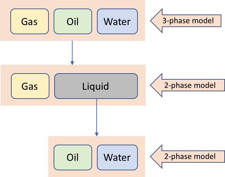
The two-phase gas-liquid model is defined in the following terms:

(10)	$\begin{array}{l}\displaystyle u_m = u_{s g} + u_{s l} = s_g u_g + (1-s_g) u_l\end{array}$

The two-phase oil-water model is defined in the following terms:

(11)	$\begin{array}{l}\displaystyle u_m = u_{s o} + u_{s w} = s_o u_o + (1-s_o-s_g) u_w\end{array}$

The 3-phase water-oil-gas model is usually built as a superposition of gas-liquid model and then oil-water model:

Mathematical Model

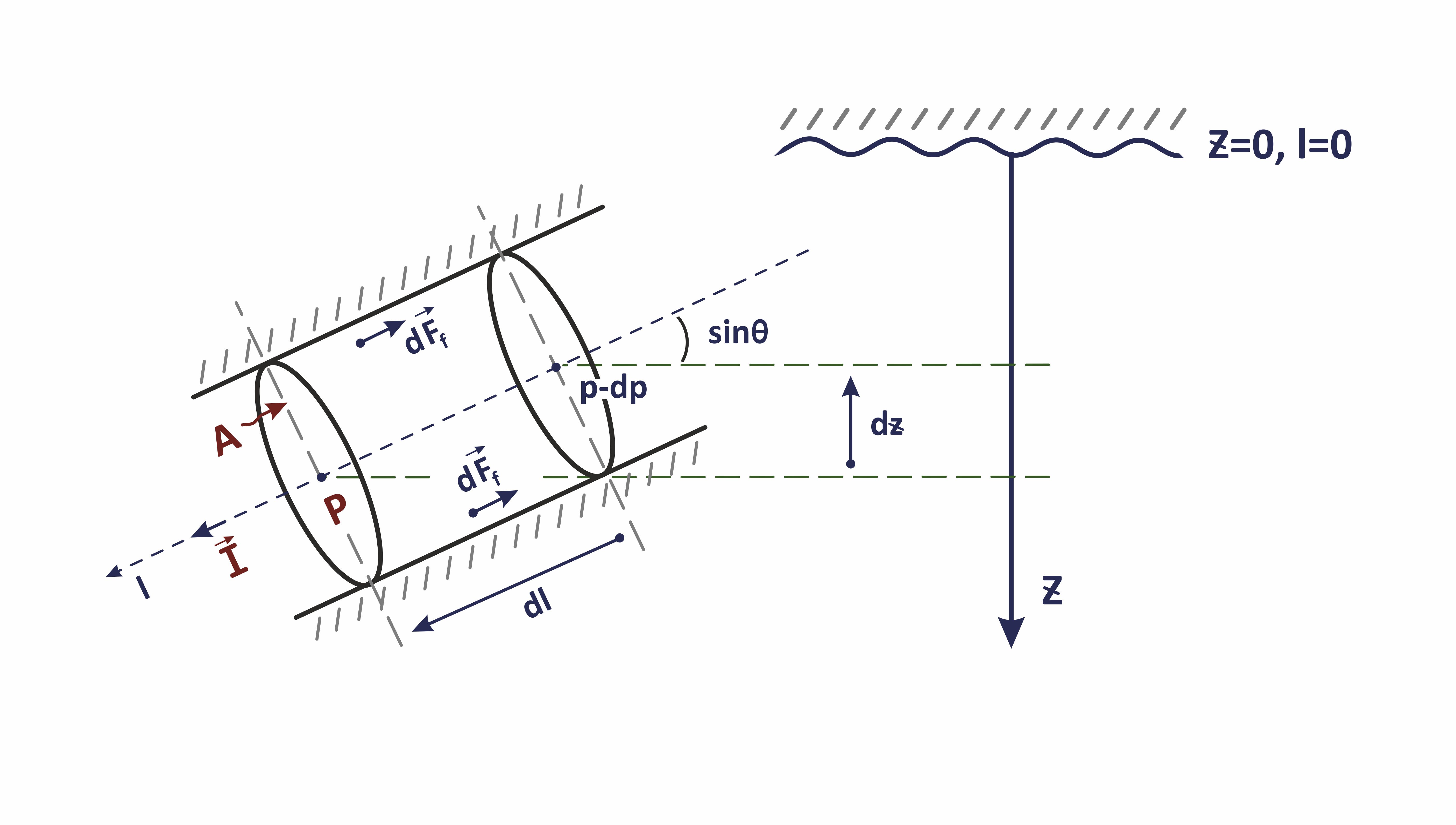
The multiphase wellbore flow in hydrodynamic and thermodynamic equilibrium is defined by the following set of 1D equations:

(12)	$\begin{array}{l}\displaystyle \frac{\partial (\rho_m A)}{\partial t} + \frac{\partial}{\partial l} \bigg( A \, \sum_\alpha \rho_\alpha \, u_\alpha \bigg) = 0\end{array}$

(13)	$\begin{array}{l}\displaystyle \sum_\alpha \rho_\alpha \bigg[ \frac{\partial u_\alpha}{\partial t} + u_\alpha \frac{\partial u_\alpha}{\partial l} - \nu_\alpha \Delta u_\alpha\bigg] = - \frac{dp}{dl} + \rho_m \, g \, \sin \theta - \frac{ f_m \, \rho_m \, u_m^2 \, }{2 d}\end{array}$

(14)

$\begin{array}{l}\displaystyle (\rho \,c_p)_m \frac{\partial T}{\partial t} - \sum_\alpha \rho_\alpha \ c_{p \alpha} \ \eta_{s \alpha} \ \frac{\partial P_\alpha}{\partial t} + \bigg( \sum_\alpha \rho_\alpha \ c_{p \alpha} \ u_\alpha \bigg) \frac{\partial T}{\partial l} \ = \ \frac{1}{A} \ \sum_\alpha \rho_\alpha \ c_{p \alpha} T_\alpha \frac{\partial q_\alpha}{\partial l}\end{array}$

where

$\begin{array}{l}m\end{array}$	indicates a mixture of fluid phases
$\begin{array}{l}\alpha = \{w,o,g \}\end{array}$	water, oil, gas phase indicator
$\begin{array}{l}l\end{array}$	measure length along wellbore trajectory
$\begin{array}{l}u_\alpha(l)\end{array}$	in-situ velocity of $\begin{array}{l}\alpha\end{array}$ -phase fluid flow
$\begin{array}{l}\rho_\alpha(l)\end{array}$	$\begin{array}{l}\alpha\end{array}$ -phase fluid density
$\begin{array}{l}\rho_m(l)\end{array}$	cross-sectional average fluid density
$\begin{array}{l}\theta(l)\end{array}$	wellbore trajectory inclination to horizon
$\begin{array}{l}d(l)\end{array}$	cross-sectional average pipe flow diameter
$\begin{array}{l}A(l)\end{array}$	in-situ cross-sectional area $\begin{array}{l}A(l) = 0.25 \, \pi \, d^2(l)\end{array}$
$\begin{array}{l}f(l)\end{array}$	Darci flow friction coefficient
$\begin{array}{l}\nu_\alpha\end{array}$	kinematic viscosity of $\begin{array}{l}\alpha\end{array}$ -phase
$\begin{array}{l}T_\alpha(l)\end{array}$	temperature of $\begin{array}{l}\alpha\end{array}$ -phase fluid flowing from reservoir into a wellbore

Equations (12) – (14) define a closed set of 3 scalar equations on 3 unknowns: pressure $\begin{array}{l}p(l)\end{array}$ , temperature $\begin{array}{l}T(l)\end{array}$ and mixture-average fluid velocity $\begin{array}{l}u_m(l)\end{array}$ .

The model is set in 1D-model with $\begin{array}{l}l-\end{array}$ axis aligned with well trajectory $\begin{array}{l}l(x,y,z)\end{array}$ :

The disambiguation of the properties in the above equation is brought in The list of dynamic flow properties and model parameters.

Equation (12) defines the continuity of the fluid components flow or equivalently represent the mass conservation of each mass component $\begin{array}{l}\{ m_W, \ m_O, \ m_G \}\end{array}$ during its transportation along wellbore.

Equation (13) defines the motion dynamics of each phase (called Navier–Stokes equation), represented as linear correlation between phase flow speed $\begin{array}{l}u_\alpha\end{array}$ and pressure profile of mutliphase fluid $\begin{array}{l}p\end{array}$ .

The term $\begin{array}{l}\sum_\alpha \rho_\alpha \ c_{p \alpha} \ u_\alpha \frac{\partial T}{\partial l}\end{array}$ represents heat convection defined by the wellbore mass flow.

The term $\begin{array}{l}\sum_\alpha \rho_\alpha \ c_{p \alpha} \ \eta_{s \alpha} \ \frac{\partial P_\alpha}{\partial t}\end{array}$ represents the heating/cooling effect of the fast adiabatic pressure change.

This usually takes effect in the wellbore during the first minutes or hours after changing the well flow regime (as a consequence of choke/pump operation).

The term $\begin{array}{l}(\rho \,c_p)_m\end{array}$ defines mass-specific heat capacity of the multiphase mixture and defined by exact formula:

(15)	$\begin{array}{l}\displaystyle (\rho \,c_p)_m = \sum_\alpha \rho_\alpha c_\alpha s_\alpha\end{array}$

The in-situ velocities $\begin{array}{l}u_\alpha\end{array}$ are usually expressed via the macroscopic flow velocity $\begin{array}{l}u_m\end{array}$ using the

Derivation

(16)

$\begin{array}{l}\displaystyle (\rho \,c_{pt})_p \frac{\partial T}{\partial t} - \sum_{a = \{w,o,g \}} \rho_\alpha \ c_{p \alpha} \ \eta_{s \alpha} \ \frac{\partial P_\alpha}{\partial t} + \sum_{a = \{w,o,g \}} \rho_\alpha \ c_{p \alpha} \ u_\alpha \frac{\partial T}{\partial l} \ = \ \frac{\delta E_H}{ \delta V \delta t}\end{array}$

Equation (14) defines the heat flow continuity or equivalently represents heat conservation due to heat conduction and convection with account for adiabatic and Joule–Thomson throttling effect.

The term $\begin{array}{l}\frac{\delta E_H}{ \delta V \delta t}\end{array}$ defines the speed of change of heat energy $\begin{array}{l}E_H\end{array}$ volumetric density due to the inflow from formation into the wellbore.

Stationary Flow Model

Stationary wellbore flow is defined as the flow with constant pressure and temperature: $\begin{array}{l}\frac{\partial T}{\partial t} = 0\end{array}$ and $\begin{array}{l}\frac{\partial P_\alpha}{\partial t} = 0\end{array}$ .

This happens during the long-term (usually hours & days & weeks) production/injection or long-term (usually hours & days & weeks) shut-in.

The temperature dynamic equation (14) is going to be:

(17)	$\begin{array}{l}\displaystyle \sum_\alpha \rho_\alpha \ c_{p \alpha} \ u_\alpha \frac{\partial T}{\partial l} \ = \ \frac{1}{A} \ \sum_\alpha \rho_\alpha \ c_{p \alpha} T_\alpha \frac{\partial q_\alpha}{\partial l}\end{array}$

The phase temperature $\begin{array}{l}T_\alpha\end{array}$ is the temperature of the $\begin{array}{l}\alpha\end{array}$ -phase flowing from reservoir into wellbore.

It carries the original reservoir temperature with heating/cooling effect from reservoir-flow throttling and well-reservoir contact throttling:

(18)	$\begin{array}{l}\displaystyle T_\alpha = T_r + \epsilon_\alpha \, \delta P = T_r + \epsilon_\alpha \, (P_e - P_{wf})\end{array}$

The discrete computational scheme for (17) will be:

(19)

$\begin{array}{l}\displaystyle \bigg( \sum_\alpha \rho_\alpha^{k-1} \ c_{p \alpha}^{k-1} \ q_\alpha^{k-1} \bigg) T^{k-1} - \bigg( \sum_\alpha \rho_\alpha^k \ c_{p \alpha}^k \ q_\alpha^k \bigg) T^k = \sum_\alpha \rho_\alpha^k \ c_{p \alpha}^k \ (q_\alpha^{k-1} - q_\alpha^k) \, (T_r^k + \epsilon_\alpha^k \delta p^k )\end{array}$

where $\begin{array}{l}\delta p^k = p_e^k - p_{wf}^k\end{array}$ is drawdown, $\begin{array}{l}p_e^k\end{array}$ – formation pressure in $\begin{array}{l}k\end{array}$ -th grid layer, $\begin{array}{l}p_{wf}^k\end{array}$ – bottom-hole pressure across $\begin{array}{l}k\end{array}$ -th grid layer, $\begin{array}{l}T_r^k\end{array}$ – remote reservoir temperature of $\begin{array}{l}k\end{array}$ -th grid layer.

The $\begin{array}{l}l\end{array}$ -axis is pointing downward along hole with $\begin{array}{l}(k-1)\end{array}$ -th grid layer sitting above the $\begin{array}{l}k\end{array}$ -th grid layer.

If the flowrate is not vanishing during the stationary lift ( $\begin{array}{l}\sum_{a = \{w,o,g \}} |q_\alpha^{k-1}| > 0\end{array}$ ) then $\begin{array}{l}T^{k-1}\end{array}$ can be calculated iteratively from previous values of the wellbore temperature $\begin{array}{l}T^k\end{array}$ as:

(20)

$\begin{array}{l}\displaystyle T^{k-1} = \frac{\bigg( \sum_\alpha \rho_\alpha^k \ c_{p \alpha}^k \ q_\alpha^k \bigg) T^k + \sum_\alpha \rho_\alpha^k \ c_{p \alpha}^k \ (q_\alpha^{k-1} - q_\alpha^k) \, (T_r^k + \epsilon_\alpha^k \delta p^k )}{\bigg( \sum_\alpha \rho_\alpha^{k-1} \ c_{p \alpha}^{k-1} \ q_\alpha^{k-1} \bigg) }\end{array}$

Deduction

(21)

$\begin{array}{l}\displaystyle (\rho \,c_{pt})_p \frac{\partial T}{\partial t} - \ \phi \sum_{a = \{w,o,g \}} \rho_\alpha \ c_{p \alpha} \ \eta_{s \alpha} \ \frac{\partial P_\alpha}{\partial t} + \bigg( \sum_{a = \{w,o,g \}} \rho_\alpha \ c_{p \alpha} \ \epsilon_\alpha \ \mathbf{u}_\alpha \bigg) \nabla P + \bigg( \sum_{a = \{w,o,g \}} \rho_\alpha \ c_{p \alpha} \ \mathbf{u}_\alpha \bigg) \ \nabla T - \nabla (\lambda_t \nabla T) = \frac{\delta E_H}{ \delta V \delta t}\end{array}$

The wellbore fluid velocity $\begin{array}{l}u_\alpha\end{array}$ can be expressed thorugh the volumetric flow profile $\begin{array}{l}q_\alpha\end{array}$ and tubing/casing cross-section area $\begin{array}{l}\pi r_f^2\end{array}$ as:

(22)	$\begin{array}{l}\displaystyle u_\alpha = \frac{q_\alpha}{\pi r_f^2}\end{array}$

so that

(23)	$\begin{array}{l}\displaystyle \bigg( \sum_{a = \{w,o,g \}} \rho_\alpha \ c_{p \alpha} \ \mathbf{u}_\alpha \bigg) \ \nabla T = \frac{\delta E_H}{ \delta V \delta t}\end{array}$

References

Beggs, H. D. and Brill, J. P.: "A Study of Two-Phase Flow in Inclined Pipes," J. Pet. Tech., May (1973), 607-617

The list of dynamic flow properties and model parameters

$\begin{array}{l}(t,x,y,z)\end{array}$	time and space corrdinates , $\begin{array}{l}z\end{array}$ -axis is orientated towards the Earth centre, $\begin{array}{l}(x,y)\end{array}$ define transversal plane to the $\begin{array}{l}z\end{array}$ -axis
$\begin{array}{l}\mathbf{r} = (x, \ y, \ z)\end{array}$	position vector at which the flow equations are set
$\begin{array}{l}l (x, \ y, \ z)\end{array}$	measured depth along borehole trajectory $\begin{array}{l}dl^2 = dx^2 + dy^2 + dz^2\end{array}$ starting from tubing head $\begin{array}{l}l (x = x_0, \ y=y_0, \ z = z_{THP}) = 0\end{array}$
$\begin{array}{l}q_{mW} = \frac{d m_W}{dt}\end{array}$	speed of water-component mass change in wellbore draining points
$\begin{array}{l}q_{mO} = \frac{d m_O}{dt}\end{array}$	speed of oil-component mass change in wellbore draining points
$\begin{array}{l}q_{mG} = \frac{d m_G}{dt}\end{array}$	speed of gas-component mass change in wellbore draining points
$\begin{array}{l}q_W = \frac{1}{\rho_W^{\LARGE \circ}} \frac{d m_W}{dt} = \frac{d V_{Ww}^{\LARGE \circ}}{dt} = \frac{1}{B_w} q_w\end{array}$	volumetric water-component flow rate in wellbore draining points recalculated to standard surface conditions
$\begin{array}{l}q_O = \frac{1}{\rho_O^{\LARGE \circ}} \frac{d m_O}{dt} = \frac{d V_{Oo}^{\LARGE \circ}}{dt} + \frac{d V_{Og}^{\LARGE \circ}}{dt} = \frac{1}{B_o} q_o + \frac{R_v}{B_g} q_g\end{array}$	volumetric oil-component flow rate in wellbore draining points recalculated to standard surface conditions
$\begin{array}{l}q_G = \frac{1}{\rho_G^{\LARGE \circ}} \frac{d m_G}{dt} = \frac{d V_{Gg}^{\LARGE \circ}}{dt} + \frac{d V_{Go}^{\LARGE \circ}}{dt} = \frac{1}{B_g} q_g + \frac{R_s}{B_o} q_o\end{array}$	volumetric gas-component flow rate in wellbore draining points recalculated to standard surface conditions
$\begin{array}{l}q_w = \frac{d V_w}{dt}\end{array}$	volumetric water-phase flow rate in wellbore draining points
$\begin{array}{l}q_o = \frac{d V_o}{dt}\end{array}$	volumetric oil-phase flow rate in wellbore draining points
$\begin{array}{l}q_g = \frac{d V_g}{dt}\end{array}$	volumetric gas-phase flow rate in wellbore draining points
$\begin{array}{l}q^S_W =\frac{dV_{Ww}^S}{dt}\end{array}$	total well volumetric water-component flow rate
$\begin{array}{l}q^S_O = \frac{d (V_{Oo}^S + V_{Og}^S )}{dt}\end{array}$	total well volumetric oil-component flow rate
$\begin{array}{l}q^S_G = \frac{d (V_{Gg}^S + V_{Go}^S )}{dt}\end{array}$	total well volumetric gas-component flow rate
$\begin{array}{l}q^S_L = q^S_W + q^S_O\end{array}$	total well volumetric liquid-component flow rate
$\begin{array}{l}\vec u_w = \vec u_w (t, \vec r)\end{array}$	water-phase flow speed distribution and dynamics
$\begin{array}{l}\vec u_o = \vec u_o (t, \vec r)\end{array}$	oil-phase flow speed distribution and dynamics
$\begin{array}{l}\vec u_g = \vec u_g (t, \vec r)\end{array}$	gas-phase flow speed distribution and dynamics
$\begin{array}{l}\vec g = (0, \ 0, \ g)\end{array}$	gravitational acceleration vector
$\begin{array}{l}g = 9.81 \ \rm m/s^2\end{array}$	gravitational acceleration constant
$\begin{array}{l}\rho_\alpha(P,T)\end{array}$	mass density of $\begin{array}{l}\alpha\end{array}$ -phase fluid
$\begin{array}{l}\mu_\alpha(P,T)\end{array}$	viscosity of $\begin{array}{l}\alpha\end{array}$ -phase fluid
$\begin{array}{l}\lambda_t(P,T,s_w, s_o, s_g)\end{array}$	effective thermal conductivity of the rocks with account for multiphase fluid saturation
$\begin{array}{l}\lambda_r(P,T)\end{array}$	rock matrix thermal conductivity
$\begin{array}{l}\lambda_\alpha(P,T)\end{array}$	thermal conductivity of $\begin{array}{l}\alpha\end{array}$ -phase fluid
$\begin{array}{l}\rho_r(P,T)\end{array}$	rock matrix mass density
$\begin{array}{l}\eta_{s \alpha}(P,T)\end{array}$	differential adiabatic coefficient of $\begin{array}{l}\alpha\end{array}$ -phase fluid
$\begin{array}{l}c_{pr}(P,T)\end{array}$	specific isobaric heat capacity of the rock matrix
$\begin{array}{l}c_{p\alpha}(P,T)\end{array}$	specific isobaric heat capacity of $\begin{array}{l}\alpha\end{array}$ -phase fluid
$\begin{array}{l}\epsilon_\alpha (P, T)\end{array}$	differential Joule–Thomson coefficient of $\begin{array}{l}\alpha\end{array}$ -phase fluid дифференциальный коэффициент Джоуля-Томсона фазы $\begin{array}{l}\alpha\end{array}$

Page tree

Wellbore Multiphase Flow

Definition

Mathematical Model

Stationary Flow Model

References

The list of dynamic flow properties and model parameters