1. Motivation

One of the most important objectives of the well testing is to assess the drainable oil reserves and reservoir properties around tested well.

This particularly becomes important in appraisal drilling as well testing is the only source of this information.

The Self-Pulse Test (SPT) is a single-well pressure test with periodic changes in flow rate and pressure (see Fig. 1).

Fig. 1. Typical record of pressure and rate variation during SPT

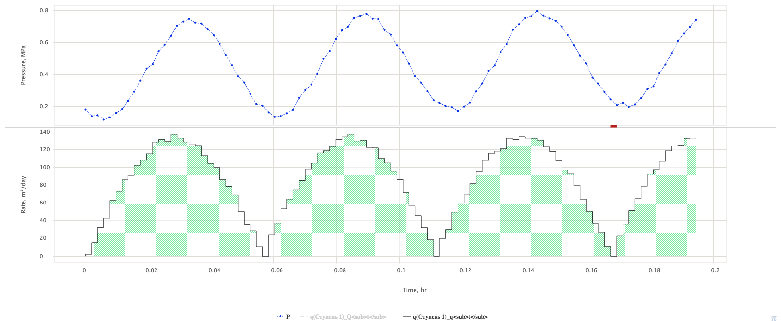
When flow rate is being intentionally varied in harmonic cycles with sandface amplitude $\begin{array}{l}q_0\end{array}$ and cycling frequency $\begin{array}{l}\omega = \frac{2 \, \pi}{T}\end{array}$ :

(1)	$\begin{array}{l}\displaystyle q(t) = q_0 \, \sin ( \omega \, t )\end{array}$

then bottom-hole pressure will follow the same variation pattern:

(2)	$\begin{array}{l}\displaystyle p_{wf}(t) = p_0 \, \sin ( \omega \, [ t - t_{\Delta} ] )\end{array}$

with a bottom-hole pressure amplitude $\begin{array}{l}p_0\end{array}$ and the time delay $\begin{array}{l}t_{\Delta}\end{array}$ .

It takes some time (3-5 cycles $\begin{array}{l}t \geq 3 \, T\end{array}$ ) for pressure to develop a stabilized response to rate variations.

The pressure delay $\begin{array}{l}t_{\Delta}\end{array}$ and associated dimensionless phase shift $\begin{array}{l}\Delta = \omega \, t_{\Delta}\end{array}$ represent the inertia effects from the adjoined reservoir and characterized by formation pressure diffusivity:

(3)	$\begin{array}{l}\displaystyle \chi = \Big < \frac{k}{\mu} \Big > \frac{1}{\phi \, c_t}\end{array}$

The diffusion nature of pressure dictates that amplitude of pressure variation is proportional to amplitude of sandface flowerate variation and the ratio $\begin{array}{l}\frac{p_0}{q_0}\end{array}$ is related to formation transmissibility:

(4)	$\begin{array}{l}\displaystyle \sigma = \Big < \frac{k}{\mu} \Big > \, h\end{array}$

The exact solution of differential diffusion equation for vertical well with negligible well storage and infinite boundary homogeneous reservoir can be represented by a system of non-linear algebraic equations, relating field-measured parameters $\begin{array}{l}\big\{ \frac{q_0}{p_0}, \, t_{\Delta} \big\}\end{array}$ to formation properties $\begin{array}{l}\{ \sigma, \, \chi \}\end{array}$ :

(5)	$\begin{array}{l}\displaystyle X =r_w \, \sqrt{ \frac{\omega}{\chi} }\end{array}$

(6)	$\begin{array}{l}\displaystyle \Delta = \omega \, t_{\Delta} = \frac{\pi}{4} - arctg{ \frac{Ker_1 X \cdot Kei \, X - Ker_1 X \cdot Kei \, X }{Ker_1 X \cdot Kei \, X +Ker_1 X \cdot Kei \, X } }\end{array}$

(7)	$\begin{array}{l}\displaystyle \sigma =\frac{1}{2 \pi} \, \frac{q_0}{p_0} \, \sqrt{ \frac{Ker^2 X + Kei^2 X}{Ker_1^2 X + Kei_1^2 X} }\end{array}$

The above equations assume that diffusivity $\begin{array}{l}\chi\end{array}$ and dimensionless radius $\begin{array}{l}X\end{array}$ are found from (5) – (6) and then $\begin{array}{l}X\end{array}$ is substituted to (7) to calculate transmissibility $\begin{array}{l}\sigma\end{array}$ .

In case of a low frequency pulsations:

(8)	$\begin{array}{l}\displaystyle \omega \ll 0.00225 \, \frac{ \chi }{ r_w^2} \quad \Longleftrightarrow \quad X \ll 0.15\end{array}$

the equations (5) – (7) can be explicitly resolved in terms of transmissibility and diffusivity:

(9)	$\begin{array}{l}\displaystyle \chi = 0.25 \, \omega \, \gamma^2 \, r_w^2 \, \exp \frac{\pi}{2 \, {\rm tg} \Delta }\end{array}$

(10)	$\begin{array}{l}\displaystyle \sigma = \frac{q_0}{8 \, p_0 \, \sin \Delta}\end{array}$

where $\begin{array}{l}\Delta = \omega \, t_{\Delta}\end{array}$ .

Expand more on analytical approach

The above analytical approach (either (5) – (7) or (9) – (10)) is rarely helpful in practise.

The field operations are very finnicky and difficult to follow the pre-desgined sequence of clean harmonic pulsations.

As result, the flowrate variation becomes a complex sum of harmonics:

(11)	$\begin{array}{l}\displaystyle q(t) = q_0 + \sum_{n=0}^\infty q_n \, \sin ( \omega_n \, t )\end{array}$

and the pressure response becomes complex as well:

(12)	$\begin{array}{l}\displaystyle p_{wf}(t) = p_0 + \sum_{n=0}^\infty p_n \, \sin ( \omega_n \, [ t - t_{\Delta_n} ] )\end{array}$

The use of analytical formulas requires fourier transformation to identify the key harmonics from the raw data with a manual control from analyst and a certain amount of subjectivism on which harmonics to pick up for calculating the transmissibility and diffusivity.

Once the harmonics are identified one need to search for the $\begin{array}{l}\{ \sigma, \, \chi \}\end{array}$ best fit to a complex system of non-linear algebraic equations:

(13)	$\begin{array}{l}\displaystyle X_n =r_w \, \sqrt{ \frac{\omega_n}{\chi} }\end{array}$

(14)	$\begin{array}{l}\displaystyle \Delta_n = \omega_n \, t_{\Delta} = \frac{\pi}{4} - arctg{ \frac{Ker_1 X_n \cdot Kei \, X_n - Ker_1 X_n \cdot Kei \, X_n }{Ker_1 X_n \cdot Kei \, X_n +Ker_1 X_n \cdot Kei \, X_n } }\end{array}$

(15)	$\begin{array}{l}\displaystyle \sigma =\frac{1}{2 \pi} \, \frac{q_n}{p_n} \, \sqrt{ \frac{Ker^2 X_n + Kei^2 X_n}{Ker_1^2 X_n + Kei_1^2 X_n} }\end{array}$

In practice, the most efficient methodology to interpret the SPT data is via fitting numerical model to the raw pressure-rate data.

Still, formulas (9) and (10) play important academic role and provide fast track estimations in SPT engineering.

2. Objectives

Assess reservoir volume around well
Assess reservoir permeability and thickness variation around well

3. Deliverables

The advantages of SPT deliverables over conventional single-well test is illustrated below.


V_hc	Potential hydrocarbon reserves
V_e	Drainage volume
A_e	Drainage area
k_near	Permeability of the near-reservoir zone
h_near	Effective thickness of the near-reservoir zone
k_far	Permeability of the far-reservoir zone
h_far	Effective thickness of the far-reservoir zone
S	Skin-factor
P_u(t)	Deconvolution of the long-term unit-rate response

BUS – Build-up Survey

Conventional single-well testing is based on long-term monitoring of downhole pressure response to the step change in flow rate (usually shut-in or close-in).

The primary hard data deliverables are:

formation pressure $\begin{array}{l}P_i\end{array}$
skin-factor S
average transmissibility in drainage area $\begin{array}{l}\sigma\end{array}$
time to reach the reservoir boundary $\begin{array}{l}t_e\end{array}$

The conditional deliverables from build-up survey would be:

Deliverables

Description

Non-BUS Input Parameters

Key Uncertainties

(16)	$\begin{array}{l}\displaystyle V_o = \frac{4 \, \sigma \, t_e \, (1-s_{wi})}{c_t}\end{array}$

where $\begin{array}{l}c_t\end{array}$ is total compressibility:

(17)	$\begin{array}{l}\displaystyle c_t = c_r + (1-s_{wi}) \, c_o + s_{wi} \, c_w\end{array}$

and $\begin{array}{l}\{ c_r, \, c_o \, c_w \}\end{array}$ are rock, oil and water compressibility.

Drainable oil reserves

The rock compressibility $\begin{array}{l}c_r(\phi)\end{array}$ is defined from core lab study or empirical porosity correlations

Fluid compressibility $\begin{array}{l}\{ c_o , \, c_w \}\end{array}$ from PVT

Initial water saturation $\begin{array}{l}s_{wi}\end{array}$ from SCAL

Rock compressibility $\begin{array}{l}c_r(\phi)\end{array}$

Initial water saturation $\begin{array}{l}s_{wi}\end{array}$

(18)	$\begin{array}{l}\displaystyle A_e = 4 \, \chi \, t_e\end{array}$

where $\begin{array}{l}\chi\end{array}$ is pressure diffusivity:

(19)	$\begin{array}{l}\displaystyle \chi = \Big< \frac{k}{\mu} \Big> \, \frac{1}{\phi \, c_t}\end{array}$

where $\begin{array}{l}\phi\end{array}$ is reservoir porosity, $\begin{array}{l}\big< \frac{k}{\mu} \big>\end{array}$ is fluid mobility:

(20)	$\begin{array}{l}\displaystyle \Big< \frac{k}{\mu} \Big> = k_a \, \bigg[ \frac{k_{rw}}{\mu_w} + \frac{k_{ro}}{\mu_o} \bigg]\end{array}$

$\begin{array}{l}k_a\end{array}$ is absolute permeability to air,

$\begin{array}{l}k_{rw}, \, k_{ro}\end{array}$ are relative permeabilities to water and oil,

$\begin{array}{l}\mu_w, \mu_o\end{array}$ are water and oil viscosities

Drainage area

Formation porosity $\begin{array}{l}\phi\end{array}$

Absolute permeability to air $\begin{array}{l}k_a\end{array}$ from core study

Relative permeabilities $\begin{array}{l}\{ k_{rw}, \, k_{ro} \}\end{array}$ from SCAL

Fluid viscosities $\begin{array}{l}\{ \mu_w, \mu_o \}\end{array}$ from PVT

Absolute permeability to air $\begin{array}{l}k_a\end{array}$

Relative permeabilities

$\begin{array}{l}\{ k_{rw}, \, k_{ro} \}\end{array}$

(21)	$\begin{array}{l}\displaystyle h = \sigma \, \bigg< \frac{k}{\mu} \bigg>^{-1}\end{array}$

Effective reservoir thickness

Absolute permeability to air $\begin{array}{l}k_a\end{array}$ from core study

Relative permeabilities $\begin{array}{l}\{ k_{rw}, \, k_{ro} \}\end{array}$ from SCAL

Fluid viscosities $\begin{array}{l}\{ \mu_w, \mu_o \}\end{array}$ from PVT

Absolute permeability to air $\begin{array}{l}k_a\end{array}$

Relative permeabilities $\begin{array}{l}\{ k_{rw}, \, k_{ro} \}\end{array}$

As one can see, the drainage area and the reservoir thickness are conditioned by core data which may not be representative of the whole drainage area.

SPT – Self-Pulse Testing

The single-well self-pulse test is based on long-term monitoring of downhole pressure response to the periodic rate step change (usually shut-in or close-in).

If flowrate

The primary hard data deliverables are:

formation pressure $\begin{array}{l}P_i\end{array}$
skin-factor S
near $\begin{array}{l}\sigma_{near}\end{array}$ and far $\begin{array}{l}\sigma_{far}\end{array}$ zone transmissibility
near $\begin{array}{l}\chi_{near}\end{array}$ and far $\begin{array}{l}\chi_{far}\end{array}$ zone pressure diffusivity
time to reach the reservoir boundary $\begin{array}{l}t_e\end{array}$

The SPT is correlating pressure variation with pre-designed flowrate variation sequence and tracks:

pressure response amplitude which depends on formation transmissibility $\begin{array}{l}\sigma\end{array}$

and

time lag between flowrate variation and pressure response which depends on formation diffusivity $\begin{array}{l}\chi\end{array}$ .

This allows estimating effective formation thickness $\begin{array}{l}h\end{array}$ directly from field survey without assumptions on core-based permeability (compare with (21)) and consequently leads to assessing the drainange area $\begin{array}{l}A_e\end{array}$ , fluid mobility $\begin{array}{l}\bigg< \frac{k}{\mu} \bigg>\end{array}$ and absolute permeability $\begin{array}{l}k_a\end{array}$ with lesser uncertainties than in BUS:

Deliverables

Description

Non-BUS Input Parameters

Key Uncertainties

(22)	$\begin{array}{l}\displaystyle h = \frac{\sigma}{\phi \, c_t \, \chi}\end{array}$

Effective reservoir thickness

Formation porosity $\begin{array}{l}\phi\end{array}$

Rock compressibility $\begin{array}{l}c_r(\phi)\end{array}$

Initial water saturation $\begin{array}{l}s_{wi}\end{array}$

Fluid compressibility $\begin{array}{l}\{ c_o , \, c_w \}\end{array}$

Rock compressibility $\begin{array}{l}c_r(\phi)\end{array}$

(23)	$\begin{array}{l}\displaystyle A_e = \frac{4 \, \sigma \, t_e}{c_t \, h}\end{array}$

Drainage area

Rock compressibility $\begin{array}{l}c_r(\phi)\end{array}$

Initial water saturation $\begin{array}{l}s_{wi}\end{array}$

Fluid compressibility $\begin{array}{l}\{ c_o , \, c_w \}\end{array}$

Rock compressibility $\begin{array}{l}c_r(\phi)\end{array}$

(24)	$\begin{array}{l}\displaystyle \Big< \frac{k}{\mu} \Big> = \chi \, \phi \, c_t\end{array}$

Fluid mobility

Rock compressibility $\begin{array}{l}c_r(\phi)\end{array}$

Initial water saturation $\begin{array}{l}s_{wi}\end{array}$

Fluid compressibility $\begin{array}{l}\{ c_o , \, c_w \}\end{array}$

Rock compressibility $\begin{array}{l}c_r(\phi)\end{array}$

Initial water saturation $\begin{array}{l}s_{wi}\end{array}$

(25)	$\begin{array}{l}\displaystyle k_a = \frac{\Big< \frac{k}{\mu} \Big>}{\bigg[ \frac{k_{rw}}{\mu_w} + \frac{k_{ro}}{\mu_o} \bigg]}\end{array}$

Absolute permeability

Rock compressibility $\begin{array}{l}c_r(\phi)\end{array}$

Initial water saturation $\begin{array}{l}s_{wi}\end{array}$

Relative permeabilities $\begin{array}{l}\{ k_{rw}, \, k_{ro} \}\end{array}$

Fluid viscosities $\begin{array}{l}\{ \mu_w, \mu_o \}\end{array}$

Fluid compressibility $\begin{array}{l}\{ c_o , \, c_w \}\end{array}$

Rock compressibility $\begin{array}{l}c_r(\phi)\end{array}$

Initial water saturation $\begin{array}{l}s_{wi}\end{array}$

Relative permeabilities $\begin{array}{l}\{ k_{rw}, \, k_{ro} \}\end{array}$

The absoluite permeability from SPT $\begin{array}{l}k_a |_{SPT}\end{array}$ is usually stacked up against core-based permeability $\begin{array}{l}k_a |_{CORE}\end{array}$ to validate the core samples and assess the effects of macroscopic features which are overlooked at core-plug size level.

Running SPT in two different cycling frequences allows assessing the near and far resevroir zones spearately.

The usual SPT workflow includes several cycling tests with different frequencies, the lower the frequency the longer the scanning range.

This captures variation of permeability and thickness when moving away from well location.

Together with deconvolution, the SPT is reproducing conventional PTA information and providing additional data on pressure diuffusivity.

This maybe used as estimation of permeability and thickness separately and their variation away from well location.

Expand more on the pressure-rate time lag in SPT

The effect of the pressure response delay $\begin{array}{l}\Delta\end{array}$ to flow rate variation in a single well test is so small (usually seconds) that conventional build-up can not capture it reliably due to a high pressure contamination and wellbore instability at early build-up times and hence pressure diffusivity normally can not be assessed.

In SPT the rate undergoes sequential step changes which allows data stacking and more accurate measurement of pressure-rate time lag and through this assess pressure diffusivity.

This effect is accurately described by analytical solution of diffusivity equation and meets practical observations.

In order to numerically reproduce a short-term pressure-rate time lag in single-well survey one needs a dedicated numerical solver since the required mesh size is very small and comparable to the well size and conventional Peaceman well model does not work (see also Numerical solutions of single-phase diffusion models).

4. Inputs

Property	Description	Data Source
B_o	Oil Formation Volume Factor	PVT samples / Correlations
Bg	Gas Formation Volume Factor	PVT samples / Correlations
B_w	Water Formation Volume Factor	PVT samples / Correlations
c_o	Oil compressibility	PVT samples / Correlations
c_w	Water compressibility	PVT samples / Correlations
cg	Gas compressibility	PVT samples / Correlations
c_r	Rock compressibility	Core samples / Correlations
s_wi	Initial water saturation	Core samples
$\begin{array}{l}\phi\end{array}$	Porosity	Core samples

5. Procedure

The typical SPT procedure is brought on Fig. 2.

Fig. 2. Typical SPT procedure

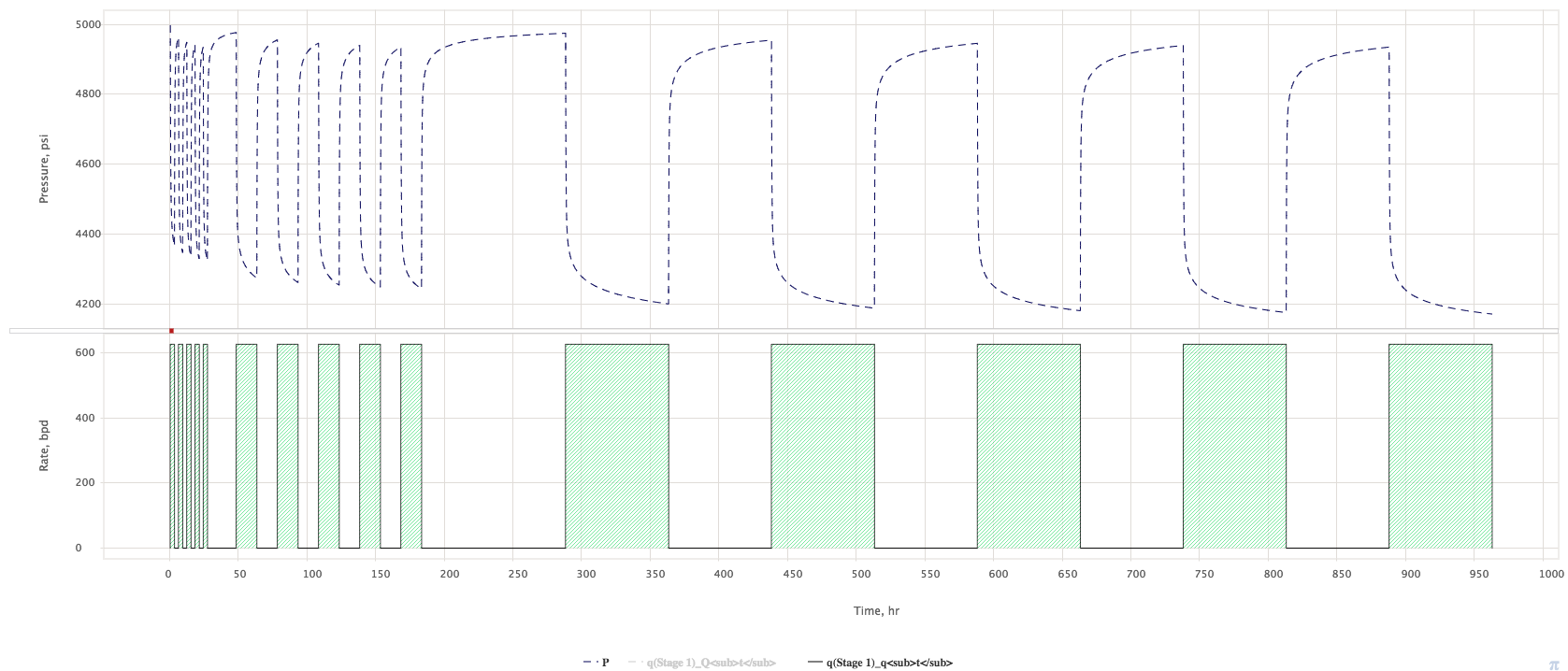
It normally consists ion three consequent tests with three different cycling frequencies:

Test 1 = high freq pulsations (10 pulses with period T)
Test 2 = mid freq pulsations (10 pulses with with period 5T)
Test 3 = Low freq pulsations (10 pulses with period 25 T)

The total duration of the test is 310 T.

Typically T = 3 hrs and total test duration is around 40 days.

Every pulse includes one choke-up and one choke-down so that full SPT survey require 60 choke operations during 40 days which is a lot of field activity for a given well.

It would be extremely difficult to perform this manually and usual practice is to arrange a programmable remote-controlled flow variation.

6. Interpretation

Numerical model
1. Single well with circle boundary
2. High density LGR
3. High density time grid (seconds)
Automated pressure match in simulation software

Page tree

1. Motivation

3. Deliverables

BUS – Build-up Survey

SPT – Self-Pulse Testing

4. Inputs

5. Procedure

6. Interpretation

References

Page tree

SPT – Self Pulse Test

1. Motivation

3. Deliverables

BUS – Build-up Survey

SPT – Self-Pulse Testing

4. Inputs

5. Procedure

6. Interpretation

References