Definition

Primary Production Analysis is the specific workflow and report template on Primary Well & Reservoir Performance Indicators.

Application

assess current production distribution
assess current distribution of recovery against expectations
assess current status and trends of recovery against expectations
assess current status and trends of reservoir depletion against expectations
assess current status and trends of water flood efficiency against expectations
quantitatively compare performance of different wells or different groups of wells
identify and prioritize redevelopment opportunities

Technology

Primary Production Analysis is built around production data against material balance and require current FDP volumetrics, PVT and SCAL models.

It includes well-by-well diagnostics and gross field diagnostics, but may be extended to sector-by-sector diagnostics.

Metrics

Primary Production Analysis includes the following metrics:

	Metric name	Diagnostic plots	Objectives
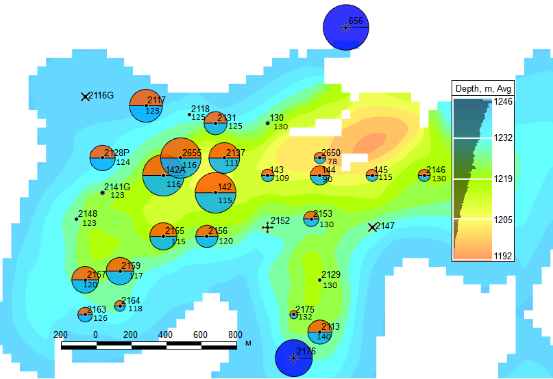
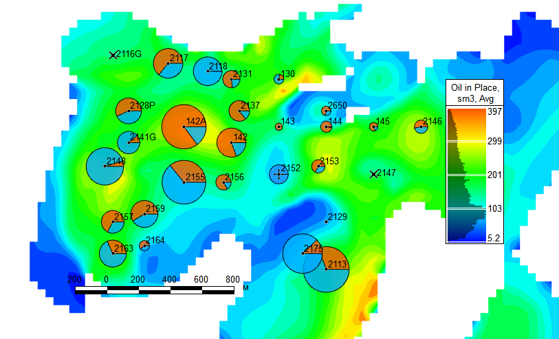
1	Production History Map	Background = Structure Bubbles = q_o, q_g , q_w, q_inj Number = CurVRR, P_e	Production Distribution Overview
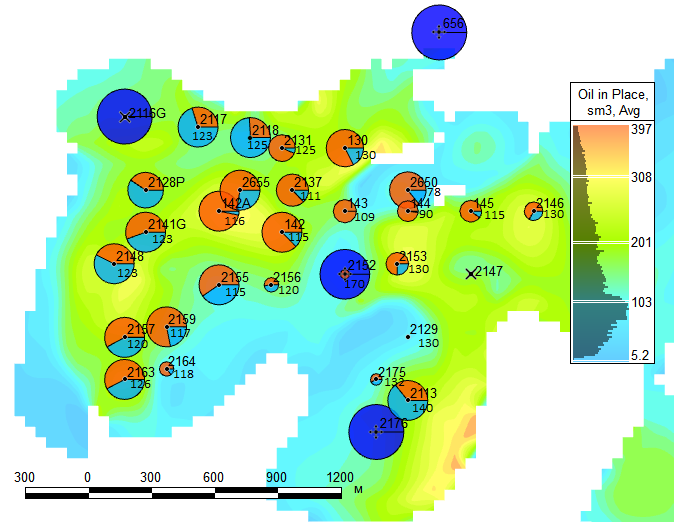
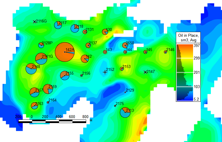
2	Recovery Map	Background = STOIIP Bubbles = Q_o, Q_g , Q_w, Q_inj Number = CumVRR, P_e	Recovery Distribution Overview
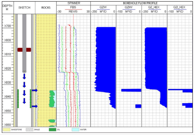
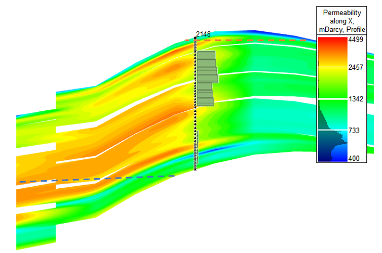
3	Cross-section	Background = STOIIP & Structure Bubbles = VRR Number = P_e , P_em
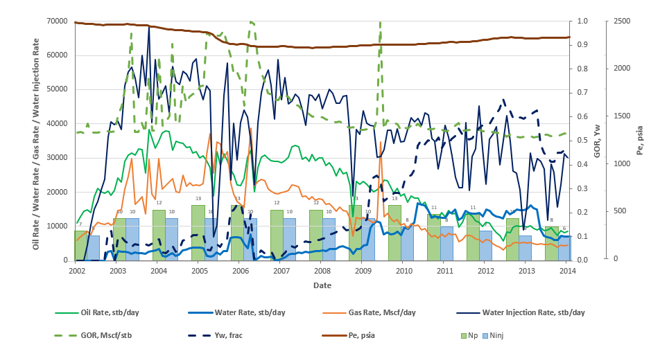
3	Production History Graphs	Left Axis = q_o, q_g , q_w, q_inj, Rigth Axis = Y_w, GOR, P_e , N_p, N_inj Hor Axis = Elapsed Time	Production History Overview
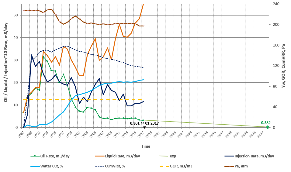
4	Decline Curve Analysis	Left Axis = q_o1, q_liq₁, q_inj1, Rigth Axis = Y_w, GOR, VRR, P_e Hor Axis = Elapsed Time	Production Forecast
5	Recovery Diagnostic	Left Axis = q_o1, q_liq₁, q_inj1 Rigth Axis =Y_w, GOR, VRR, P_e, P_em Hor Axis = RF	Estimate recovery efficiency and pressure decline
6	Watercut Diagnostic	Left Axis = Y_w, Y_wm Hor Axis = q_liq	Check for water balance and thief water production
7	GOR Diagnostic	Left Axis = GOR, GOR_gm Hor Axis =q_o	Check for gas balance and thief gas production
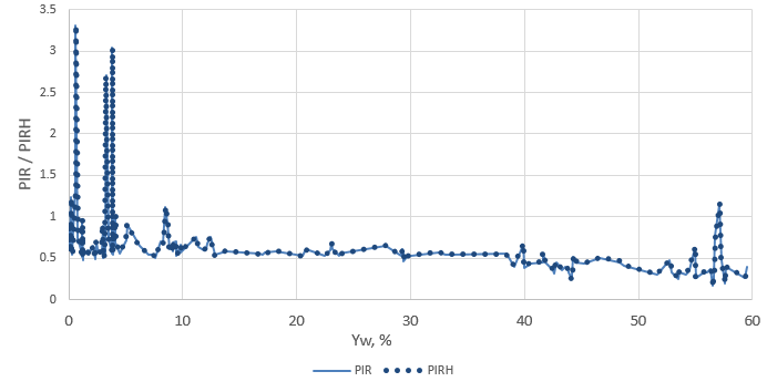
8	Injection Efficiency Diagnostics	Left Axis = PIR , PIR_m Hor Axis = Y_w	Evaluate WI efficiency
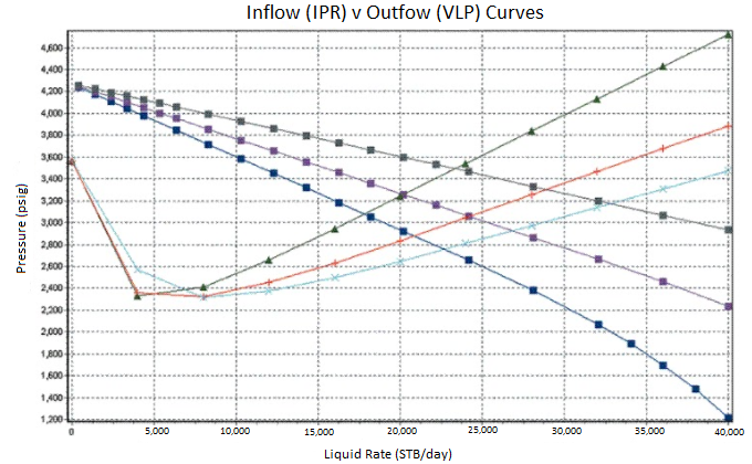
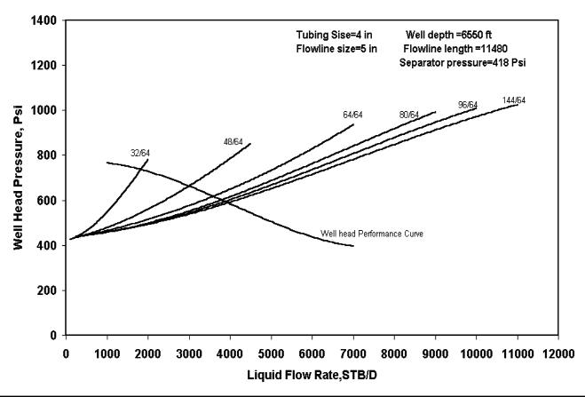
9	Well Performance Analysis	Left Axis = P_{wf_IPR} , P_{wf_VLP} Hor Axis = q_o	Check for the optimal production/injection target
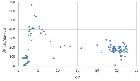
10	Productivity Index Diagnostic	Left Axis = J_PI, J_PIm Hor Axis = dP = P_wf - P_e	Check for PI dynamics

Below is the list of the production properties involved in the above metrics.

Property Abbrevy

Property Name

Formula

VRR_cum

Cumulative Voidage Replacement Ratio

(1)	$\begin{array}{l}\displaystyle {\rm VRR_{cum}} = \frac{B_w \, Q_{WI}}{B_w \, Q_W + B_o \, Q_O + B_g Q_G - B_g R_s Q_O}\end{array}$

VRRcur

Current Voidage Replacement Ratio

(month over month)

(2)	$\begin{array}{l}\displaystyle {\rm VRR_{cur}} = \frac{B_w \, q_{WI}}{B_w \, q_W + B_o \, q_O + B_g (q_G - R_s Q_O)}\end{array}$

RF

Recovery Factor

(3)	$\begin{array}{l}\displaystyle {\rm RF} = \frac{Q_O}{V_{STOIIP}}\end{array}$

Y_w

Watercut (production)

(4)	$\begin{array}{l}\displaystyle {\rm Y_w} = \frac{q_W}{q_{LIQ}}\end{array}$

Y_wm

Watercut (proxy-model)

(5)	$\begin{array}{l}\displaystyle {\rm Y_{wm}} = \frac{1}{1 + \frac{K_{ro}}{K_{rw}} \cdot \frac{ \mu_w}{\mu_o} \cdot \frac{B_w}{B_o} }\end{array}$

(6)	$\begin{array}{l}\displaystyle s_w = \frac{Q_o \, B_o}{V_\phi}\end{array}$

GOR

Gas-Oil Ratio (production)

(7)	$\begin{array}{l}\displaystyle {\rm GOR} = \frac{q_g}{q_o}\end{array}$

GOR_m

Gas-Oil Ratio (proxy-model)

(8)	$\begin{array}{l}\displaystyle {\rm GOR_m} = R_s + \frac{k_{rg}}{k_{ro}} \cdot \frac{\mu_o}{\mu_g} \cdot \frac{B_o }{B_g}\end{array}$

q_LIQ

Liquid rate

(9)	$\begin{array}{l}\displaystyle q_{LIQ} = q_O + q_W\end{array}$

PIR

Production Injection Ratio (production)

(10)	$\begin{array}{l}\displaystyle {\rm PIR} = \frac{Q_O}{Q_{WI}}\end{array}$

PIR_m

Production Injection Ratio (model)

(11)	$\begin{array}{l}\displaystyle {\rm PIR_m} = { \frac{1}{VRR} } \cdot { \frac{1-Y_w}{ Y_w + (1-Y_w) \bigg[ \frac{B_o}{B_w} - \frac{B_g}{B_w}(GOR - R_s) \bigg] } }\end{array}$

J_O

Oil Productivity Index

(12)	$\begin{array}{l}\displaystyle {\rm J_{O}} = \frac{q_O}{P_e - P_{wf}} {\quad \Rightarrow \quad} P_{wf} = P_e - \frac{1}{J_O} q_O\end{array}$

J_PI

Total Productivity Index (production)

(13)	$\begin{array}{l}\displaystyle {\rm J_t} = \frac{q_t}{P_e - P_{wf}}\end{array}$

J_PIm

Total Productivity Index (model)

(14)	$\begin{array}{l}\displaystyle {\rm J_{tm} } = \frac{2 \pi \sigma}{\ln \frac{r_e}{r_w} +0.5 + S}\end{array}$

PIR equation deduction

(15)	$\begin{array}{l}\displaystyle VRR = \frac{B_w \, q_{WI}}{B_w \, q_W + B_o \, q_O + B_g \, [ q_G - R_s \, q_O] } = \frac{B_w \, q_{WI}}{B_w \, q_W + B_o \, q_O + B_g \, [ GOR - R_s] q_O } = \frac{B_w \, q_{WI}}{B_w \, q_W + [ B_o + B_g \, ( GOR - R_s) ] \, q_O }\end{array}$

(16)	$\begin{array}{l}\displaystyle VRR = \frac{q_{WI}}{q_W + \bigg[ \frac{B_o}{B_w} + \frac{B_g}{B_w} \, ( GOR - R_s) \bigg] \, q_O }\end{array}$

(17)	$\begin{array}{l}\displaystyle Y_w=\frac{q_W}{q_W + q_O} \rightarrow \frac{q_O}{q_W} = \frac{1-Y_w}{Y_w} \rightarrow q_W = \frac{Y_w}{1-Y_w} \, q_O\end{array}$

(18)	$\begin{array}{l}\displaystyle VRR = \frac{q_{WI}}{q_O} \cdot \frac{1}{\frac{Y_w}{1-Y_w} + \bigg[ \frac{B_o}{B_w} + \frac{B_g}{B_w} \, ( GOR - R_s) \bigg] } = \frac{q_{WI}}{q_O} \cdot \frac{1-Y_w}{Y_w + (1-Y_w) \, \bigg[ \frac{B_o}{B_w} + \frac{B_g}{B_w} \, ( GOR - R_s) \bigg] }\end{array}$

(19)	$\begin{array}{l}\displaystyle PIR=\frac{q_W}{q_{WI}} = \frac{1}{VRR} \cdot \frac{1-Y_w}{Y_w + (1-Y_w) \, \bigg[ \frac{B_o}{B_w} + \frac{B_g}{B_w} \, ( GOR - R_s) \bigg] }\end{array}$

Diagnostic

Expand

Sample Case 1 – Sector Analysis


Fig. 1. Production History Map	Fig. 2. Recovery Map	Fig. 3. Cross-section & PLT, permeability, GOC, OWC


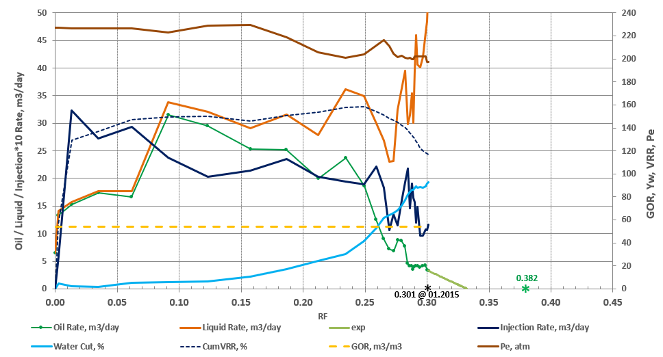Fig. 4. Production History Graphs	Fig. 5. Decline Curve Analysis	Fig. 6. Recovery Diagnostic


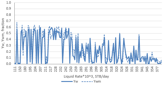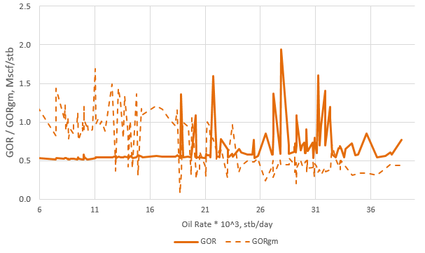Fig. 7. Watercut Diagnostic	Fig. 8. GOR Diagnostic	Fig. 9. Injection Efficiency Diagnostics


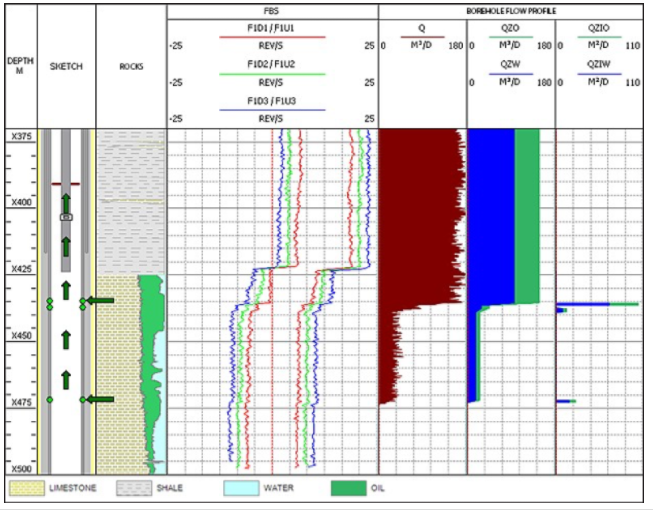
Fig. 10. Well Performance Analysis (VFP + IPR)	Fig. 11. Productivity Index Diagnostic	Fig. 12. Well Completion & PLT

Sample Case 2 – Producer Analysis


Fig. 1. Production History Map	Fig. 2. Recovery Map	Fig. 3. Cross-section & PLT


Fig. 4. Production History Graphs	Fig. 5. Decline Curve Analysis	Fig. 6. Recovery Diagnostic


Fig. 7. Watercut Diagnostic	Fig. 8. GOR Diagnostic	Fig. 9. Injection Efficiency Diagnostics


Fig. 10. Well Performance Analysis (VFP + IPR)	Fig. 11. Productivity Index Diagnostic	Fig. 12. Well Completion & PLT

Sample Case 3 – Injector Analysis


Fig. 1. Production History Map	Fig. 2. Recovery Map	Fig. 3. Cross-section & PLT


Fig. 4. Production History Graphs


Fig. 10. Well Performance Analysis (VFP + IPR)	Fig. 11. Injectivity Index Diagnostic	Fig. 12. Well Completion & PLT

Page tree

PRIME – Primary Production Analysis