| Expand | |||||||||||||||||||||
|---|---|---|---|---|---|---|---|---|---|---|---|---|---|---|---|---|---|---|---|---|---|
| |||||||||||||||||||||
|
Motivation
Assume the well is producing
| LaTeX Math Inline | ||
|---|---|---|
|
| LaTeX Math Inline | ||
|---|---|---|
|
| LaTeX Math Inline | ||
|---|---|---|
|
| LaTeX Math Inline | ||
|---|---|---|
|
| LaTeX Math Inline | ||
|---|---|---|
|
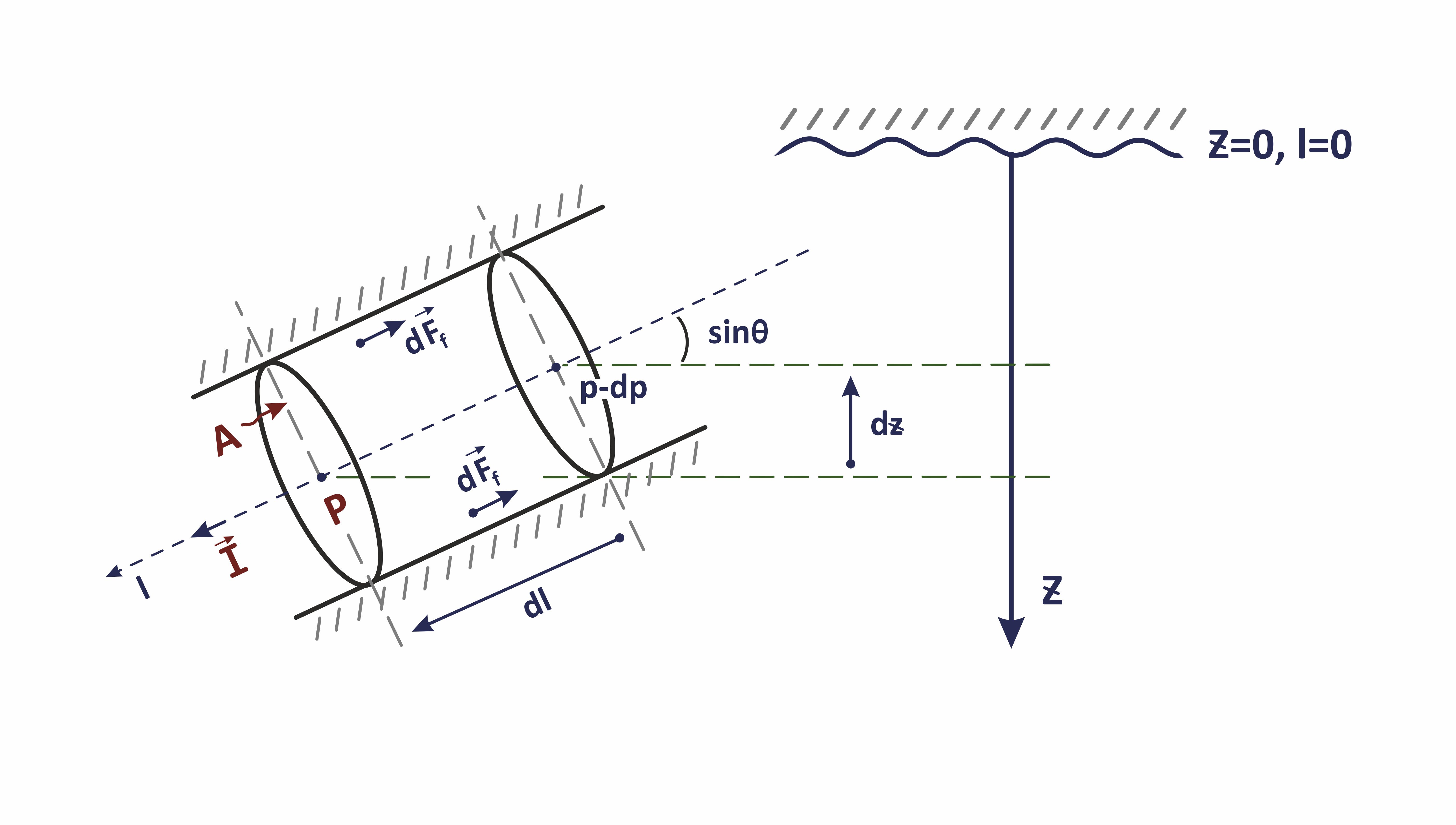
While going down to depth
| LaTeX Math Inline | ||
|---|---|---|
|
| LaTeX Math Inline | ||
|---|---|---|
|
Wellbore temperature
| LaTeX Math Inline | ||
|---|---|---|
|
The volume shares
| LaTeX Math Inline | ||
|---|---|---|
|
It is now possible to simulate the stationary multiphase wellbore flow and link the surface flow conditions (pressure, temperature and rates) to downhole flow conditions at any depth.
| Expand | ||
|---|---|---|
| ||
|
The most adequate and practical model can be built for a stationary fluid flow at hydrodynamic and thermodynamic equilibrium.
If flow is changing slowly over time the same solutions can be used with inputs as time functions which is called quasi-stationary flow conditions.
This model finds important applications in industry.
If well production has been changed abruptly (for example opening or closing the flow) there will be a transition period towards the new quasi-stationary flow conditions (usually minutes or few hours).
The transition period for pressure and temperature is different and wellbore temperature takes much longer time to stabilize than pressure.
Unlike single-phase flow (Wellbore Water Flow and Wellbore Gas Flow) the complexity of the multiphase flow during transition is so high and unstable that building a simple mathematical model does not make a practical sense.
Definition
Mathematical model of Multiphase Wellbore Flow predicts the temperature, pressure and flow speed distribution along the wellbore trajectory with account for:
- tubing head pressure which is controled by gathering system or injection pump
- wellbore design (pipe diameters, pipe materials and inter-pipe annular fillings)
- fluid friction with tubing /casing walls
- interfacial phase slippage
- heat exchange between wellbore fluid and surrounding rocks via complex well design
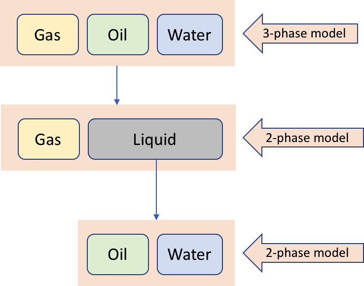
Consider a 3-phase water-oil-gas flow:
| LaTeX Math Inline | ||
|---|---|---|
|
The
| LaTeX Math Inline | ||
|---|---|---|
|
| LaTeX Math Block | ||||
|---|---|---|---|---|
| ||||
\gamma_\alpha = \frac{q_\alpha}{q_t} |
where
| LaTeX Math Inline | ||
|---|---|---|
|
| LaTeX Math Inline | ||
|---|---|---|
|
| LaTeX Math Inline | ||
|---|---|---|
|
| LaTeX Math Block | ||||
|---|---|---|---|---|
| ||||
q_t = \sum_\alpha q_\alpha = q_w + q_o + g_g |
In multiphase wellbore flow each phase occupies its own area
| LaTeX Math Inline | ||
|---|---|---|
|
| LaTeX Math Inline | ||
|---|---|---|
|
This area can be connected into a single piece of cross-sectional area (like in case of slug or annular flow) or dispersed into a number of connected spots (like in case of bubbly flow).
A share of total pipe cross-section area occupied by moving
| LaTeX Math Inline | ||
|---|---|---|
|
| LaTeX Math Inline | ||
|---|---|---|
|
| LaTeX Math Block | ||||
|---|---|---|---|---|
| ||||
s_\alpha = \frac{A_\alpha}{A} |
so that a sum of all in-situ hold-ups is subject to natural constraint:
| LaTeX Math Block | ||||
|---|---|---|---|---|
| ||||
\sum_\alpha s_\alpha = s_w + s_o + s_g = 1 |
When word hold-up is used alone it usually means in-situ hold-up and should not be confused with input hold-up or no-slip hold-up which should be better called volumetric flow fraction.
The actual average cross-sectional velocity of moving
| LaTeX Math Inline | ||
|---|---|---|
|
| LaTeX Math Block | ||||
|---|---|---|---|---|
| ||||
u_\alpha = \frac{q_\alpha}{A_\alpha} |
where
| LaTeX Math Inline | ||
|---|---|---|
|
| LaTeX Math Inline | ||
|---|---|---|
|
| LaTeX Math Inline | ||
|---|---|---|
|
The superficial velocity of
| LaTeX Math Inline | ||
|---|---|---|
|
| LaTeX Math Block | ||||
|---|---|---|---|---|
| ||||
u_{s \alpha} = \frac{q_\alpha}{A}= s_\alpha \cdot u_\alpha |
The multiphase mixture velocity is defined as total flow volume normalized by the total cross-sectional area:
| LaTeX Math Block | ||||
|---|---|---|---|---|
| ||||
u_m = \frac{1}{A} \sum_\alpha q_\alpha = \sum_\alpha u_{s \alpha} = \sum_\alpha s_\alpha \cdot u_\alpha |
The difference between velocities of
| LaTeX Math Inline | ||
|---|---|---|
|
| LaTeX Math Inline | ||
|---|---|---|
|
| LaTeX Math Block | ||||
|---|---|---|---|---|
| ||||
u_{\alpha_1 \alpha_2} = u_{\alpha_1} - u_{\alpha_2} |
The multiphase fluid density
| LaTeX Math Inline | ||
|---|---|---|
|
| LaTeX Math Block | ||||
|---|---|---|---|---|
| ||||
\rho_m = \sum_\alpha s_\alpha \rho_\alpha |
where
| LaTeX Math Inline | ||
|---|---|---|
|
| LaTeX Math Inline | ||
|---|---|---|
|
The two-phase gas-liquid model is defined in the following terms:
| LaTeX Math Block | ||||
|---|---|---|---|---|
| ||||
u_m = u_{s g} + u_{s l} = s_g u_g + (1-s_g) u_l |
The two-phase oil-water model is defined in the following terms:
| LaTeX Math Block | ||||
|---|---|---|---|---|
| ||||
u_m = u_{s o} + u_{s w} = s_o u_o + (1-s_o-s_g) u_w |
The 3-phase water-oil-gas model is usually built as a superposition of gas-liquid model and then oil-water model:
Input & Output
| Input | Output | ||||||||
|---|---|---|---|---|---|---|---|---|---|
|
|
| Anchor | ||||
|---|---|---|---|---|
|
Application
| Activity | Input | Output | ||||||||||
|---|---|---|---|---|---|---|---|---|---|---|---|---|
| 1 | WPA – Well Performance Analysis | Optimizing the lift performance based on the IPR vs VLP models |
|
| ||||||||
| 2 | DM – Dynamic Modelling | Relating production rates at separator to bottom-hole pressure with VLP |
|
| ||||||||
| 3 | PRT – Pressure Testing | Adjust gauge pressure to formation datum |
|
| ||||||||
| 4 | PLT – Production Logging | Interpretation of production logs |
|
| ||||||||
| 5 | RFP – Reservoir Flow Profiling | Interpretation of reservoir flow logs |
|
|
Mathematical Model
Homogeneous Model
The multiphase homogeneous wellbore flow model assumes that fluid is at stationary hydrodynamic and thermodynamic equilibrium and there is no slip between phases.
This means that all have the same temperature:
| LaTeX Math Block | ||||
|---|---|---|---|---|
| ||||
T_w = T_o = T_g = T |
same pressure:
| LaTeX Math Block | ||||
|---|---|---|---|---|
| ||||
P_w = P_o = P_g = T |
same velocity:
| LaTeX Math Block | ||||
|---|---|---|---|---|
| ||||
u_w = u_o = u_g = u_m |
and all dynamic fluid parameters are constant in time:
| LaTeX Math Block | ||||
|---|---|---|---|---|
| ||||
\frac{\partial T}{\partial t} = 0, \quad \frac{\partial P}{\partial t} = 0, \quad \frac{\partial u_m}{\partial t} = 0 |
The model is defined by the following set of 1D equations:
| LaTeX Math Block | ||||
|---|---|---|---|---|
| ||||
A(l) \rho_m u_m = \rho_{sm} q_{s} = \rm const |
| LaTeX Math Block | ||||
|---|---|---|---|---|
| ||||
\frac{dp}{dl} = - \rho_m u_m \frac{\partial u_m}{\partial l} + \rho_m \, g \, \cos \theta + \frac{ f_m \, \rho_m \, u_m^2 \, }{2 d} |
| LaTeX Math Block | ||||
|---|---|---|---|---|
| ||||
\sum_\alpha \big( \rho_\alpha \, c_{p \, \alpha}  \big) \ q_m \  \frac{\partial T}{\partial l}
\ = \ \sum_\alpha \rho_\alpha \ c_{p \alpha} T_\alpha \frac{\partial q_\alpha}{\partial l} |
The right side of equation
| LaTeX Math Block Reference | ||
|---|---|---|
|
| LaTeX Math Inline | ||
|---|---|---|
|
| LaTeX Math Block | ||||
|---|---|---|---|---|
| ||||
T_\alpha = T_r + \epsilon_\alpha \, \delta p = T_r + \epsilon_\alpha \, (p_e - p) |
The discrete computational scheme for
| LaTeX Math Block Reference | ||
|---|---|---|
|
| LaTeX Math Block | ||||
|---|---|---|---|---|
| ||||
\bigg( \sum_\alpha \rho_\alpha^{k-1} \ c_{p \alpha}^{k-1} \ q_\alpha^{k-1} \bigg) T^{k-1} - \bigg( \sum_\alpha \rho_\alpha^k \ c_{p \alpha}^k \ q_\alpha^k \bigg) T^k
= \sum_\alpha \rho_\alpha^k \ c_{p \alpha}^k \ (q_\alpha^{k-1} - q_\alpha^k) \, (T_r^k + \epsilon_\alpha^k \delta p^k ) |
where
| LaTeX Math Inline | ||
|---|---|---|
|
| LaTeX Math Inline | ||
|---|---|---|
|
| LaTeX Math Inline | ||
|---|---|---|
|
| LaTeX Math Inline | ||
|---|---|---|
|
| LaTeX Math Inline | ||
|---|---|---|
|
| LaTeX Math Inline | ||
|---|---|---|
|
| LaTeX Math Inline | ||
|---|---|---|
|
The
| LaTeX Math Inline | ||
|---|---|---|
|
| LaTeX Math Inline | ||
|---|---|---|
|
| LaTeX Math Inline | ||
|---|---|---|
|
If the flowrate is not vanishing during the stationary lift (
| LaTeX Math Inline | ||
|---|---|---|
|
| LaTeX Math Inline | ||
|---|---|---|
|
| LaTeX Math Inline | ||
|---|---|---|
|
| LaTeX Math Block | ||||
|---|---|---|---|---|
| ||||
T^{k-1} = \frac{\bigg( \sum_\alpha \rho_\alpha^k \ c_{p \alpha}^k \ q_\alpha^k \bigg) T^k + \sum_\alpha \rho_\alpha^k \ c_{p \alpha}^k \ (q_\alpha^{k-1} - q_\alpha^k) \, (T_r^k + \epsilon_\alpha^k \delta p^k )}{\bigg( \sum_\alpha \rho_\alpha^{k-1} \ c_{p \alpha}^{k-1} \ q_\alpha^{k-1} \bigg) }
|
Slippage Model
The multiphase slippage wellbore flow model assumes that fluid is at hydrodynamic and thermodynamic equilibrium and there is a slip between phases so that phases may be moving with different flow speeds
| LaTeX Math Inline | ||
|---|---|---|
|
The model is defined by the following set of 1D equations:
| LaTeX Math Block | ||||
|---|---|---|---|---|
| ||||
A(l) \sum_\alpha \rho_\alpha u_\alpha = \sum_\alpha \rho_{s\alpha} q_{s\alpha} = \rm const |
| LaTeX Math Block | ||||
|---|---|---|---|---|
| ||||
\sum_\alpha \rho_\alpha u_\alpha \frac{\partial u_\alpha}{\partial l} = - \frac{dp}{dl} + \rho_m \, g \, \cos \theta + \frac{ f_m \, \rho_m \, u_m^2 \, }{2 d} |
| LaTeX Math Block | ||||
|---|---|---|---|---|
| ||||
\sum_\alpha \rho_\alpha \ c_{p \alpha} \ u_\alpha \frac{\partial T}{\partial l}
\ = \ \frac{1}{A} \ \sum_\alpha \rho_\alpha \ c_{p \alpha} T_\alpha \frac{\partial q_\alpha}{\partial l} |
It carries the original reservoir temperature with heating/cooling effect from reservoir-flow throttling and well-reservoir contact throttling:
| LaTeX Math Block | ||||
|---|---|---|---|---|
| ||||
T_\alpha = T_r + \epsilon_\alpha \, \delta P = T_r + \epsilon_\alpha \, (P_e - P_{wf}) |
see Nomenclature below.
References
| Anchor | ||||
|---|---|---|---|---|
|
Nomenclature
| position vector at which the flow equations are set | ||||||||||||||||||||||
| time and space corrdinates ,
| ||||||||||||||||||||||
| measured depth along wellbore trajectory
| ||||||||||||||||||||||
| indicates a mixture of fluid phases | ||||||||||||||||||||||
| water, oil, gas phase indicator |
| differential Joule–Thomson coefficient of
| ||||||||||||||||||||
| pressure at separator |
| differential adiabatic coefficient of
| ||||||||||||||||||||
| temperature at separator |
| Darcy friction factor at fluid velocity
| ||||||||||||||||||||
| wellbore fluid pressure |
| cross-sectional average pipe flow diameter | ||||||||||||||||||||
| wellbore fluid temperature |
| cross-sectional area
| ||||||||||||||||||||
| volumetric flow rate
|
| wellbore trajectory inclination to horizon | ||||||||||||||||||||
| in-situ velocity of
|
| gravitational acceleration constant | ||||||||||||||||||||
|
|
| effective thermal conductivity of the rocks with account for multiphase fluid saturation | ||||||||||||||||||||
| cross-sectional average fluid density |
| rock matrix thermal conductivity | ||||||||||||||||||||
| kinematic viscosity of
|
| thermal conductivity of | ||||||||||||||||||||
| dynamic viscosity of
|
| rock matrix mass density | ||||||||||||||||||||
| specific isobaric heat capacity of
|
| specific isobaric heat capacity of the rock matrix | ||||||||||||||||||||