| Expand | |||||||||||||||||||||
|---|---|---|---|---|---|---|---|---|---|---|---|---|---|---|---|---|---|---|---|---|---|
| |||||||||||||||||||||
|
Motivation
Assume the well is producing
| LaTeX Math Inline | ||
|---|---|---|
|
| LaTeX Math Inline | ||
|---|---|---|
|
| LaTeX Math Inline | ||
|---|---|---|
|
| LaTeX Math Inline | ||
|---|---|---|
|
| LaTeX Math Inline | ||
|---|---|---|
|
While going down to depth
| LaTeX Math Inline | ||
|---|---|---|
|
| LaTeX Math Inline | ||
|---|---|---|
|
Wellbore temperature
| LaTeX Math Inline | ||
|---|---|---|
|
The volume shares
| LaTeX Math Inline | ||
|---|---|---|
|
It is now possible to simulate the stationary multiphase wellbore flow and link the surface flow conditions (pressure, temperature and rates) to downhole flow conditions at any depth.
| Expand | ||
|---|---|---|
| ||
|
The most adequate and practical model can be built for a stationary fluid flow at hydrodynamic and thermodynamic equilibrium.
If flow is changing slowly over time the same solutions can be used with inputs as time functions which is called quasi-stationary flow conditions.
This model finds important applications in industry.
If well production has been changed abruptly (for example opening or closing the flow) there will be a transition period towards the new quasi-stationary flow conditions (usually minutes or few hours).
The transition period for pressure and temperature is different and wellbore temperature takes much longer time to stabilize than pressure.
Unlike single-phase flow (Wellbore Water Flow and Wellbore Gas Flow) the complexity of the multiphase flow during transition is so high and unstable that building a simple mathematical model does not make a practical sense.
Definition
Mathematical model of Multiphase Wellbore Flow predicts the temperature, pressure and flow speed distribution along the wellbore trajectory with account for:
- tubing head pressure which is controled by gathering system or injection pump
- wellbore design (pipe diameters, pipe materials and inter-pipe annular fillings)
- fluid friction with tubing /casing walls
- interfacial phase slippage
- heat exchange between wellbore fluid and surrounding rocks via complex well design
Consider a 3-phase water-oil-gas flow:
| LaTeX Math Inline | ||
|---|---|---|
|
The
| LaTeX Math Inline | ||
|---|---|---|
|
| LaTeX Math Block | ||||
|---|---|---|---|---|
| ||||
\gamma_\alpha = \frac{q_\alpha}{q_t} |
where
| LaTeX Math Inline | ||
|---|---|---|
|
| LaTeX Math Inline | ||
|---|---|---|
|
| LaTeX Math Inline | ||
|---|---|---|
|
| LaTeX Math Block | ||||
|---|---|---|---|---|
| ||||
q_t = \sum_\alpha q_\alpha = q_w + q_o + g_g |
In multiphase wellbore flow each phase occupies its own area
| LaTeX Math Inline | ||
|---|---|---|
|
| LaTeX Math Inline | ||
|---|---|---|
|
This area can be connected into a single piece of cross-sectional area (like in case of slug or annular flow) or dispersed into a number of connected spots (like in case of bubbly flow).
A share of total pipe cross-section area occupied by moving
| LaTeX Math Inline | ||
|---|---|---|
|
| LaTeX Math Inline | ||
|---|---|---|
|
| LaTeX Math Block | ||||
|---|---|---|---|---|
| ||||
s_\alpha = \frac{A_\alpha}{A} |
so that a sum of all in-situ hold-ups is subject to natural constraint:
| LaTeX Math Block | ||||
|---|---|---|---|---|
| ||||
\sum_\alpha s_\alpha = s_w + s_o + s_g = 1 |
When word hold-up is used alone it usually means in-situ hold-up and should not be confused with input hold-up or no-slip hold-up which should be better called volumetric flow fraction.
The actual average cross-sectional velocity of moving
| LaTeX Math Inline | ||
|---|---|---|
|
| LaTeX Math Block | ||||
|---|---|---|---|---|
| ||||
u_\alpha = \frac{q_\alpha}{A_\alpha} |
where
| LaTeX Math Inline | ||
|---|---|---|
|
| LaTeX Math Inline | ||
|---|---|---|
|
| LaTeX Math Inline | ||
|---|---|---|
|
The superficial velocity of
| LaTeX Math Inline | ||
|---|---|---|
|
| LaTeX Math Block | ||||
|---|---|---|---|---|
| ||||
u_{s \alpha} = \frac{q_\alpha}{A}= s_\alpha \cdot u_\alpha |
The multiphase mixture velocity is defined as total flow volume normalized by the total cross-sectional area:
| LaTeX Math Block | ||||
|---|---|---|---|---|
| ||||
u_m = \frac{1}{A} \sum_\alpha q_\alpha = \sum_\alpha u_{s \alpha} = \sum_\alpha s_\alpha \cdot u_\alpha |
The difference between velocities of
| LaTeX Math Inline | ||
|---|---|---|
|
| LaTeX Math Inline | ||
|---|---|---|
|
| LaTeX Math Block | ||||
|---|---|---|---|---|
| ||||
u_{\alpha_1 \alpha_2} = u_{\alpha_1} - u_{\alpha_2} |
The multiphase fluid density
| LaTeX Math Inline | ||
|---|---|---|
|
| LaTeX Math Block | ||||
|---|---|---|---|---|
| ||||
\rho_m = \sum_\alpha s_\alpha \rho_\alpha |
where
| LaTeX Math Inline | ||
|---|---|---|
|
| LaTeX Math Inline | ||
|---|---|---|
|
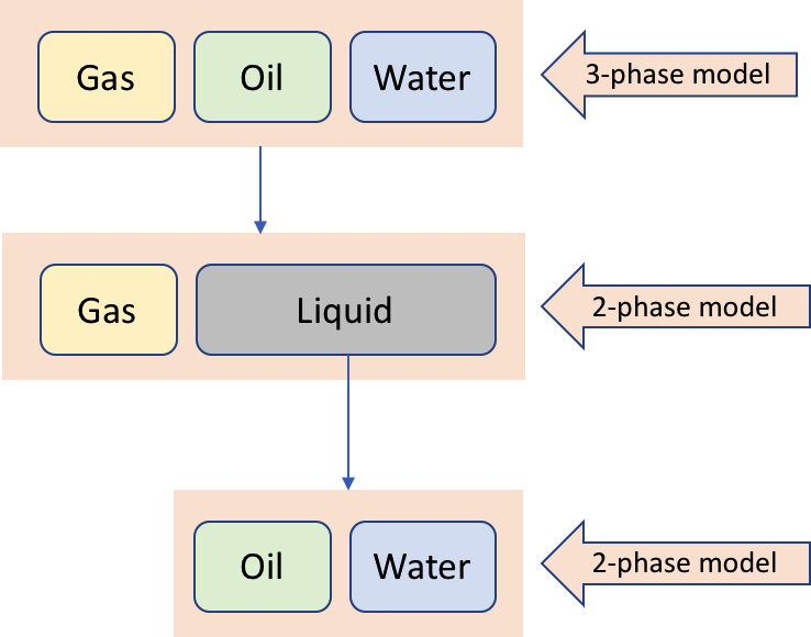
The two-phase gas-liquid model is defined in the following terms:
| LaTeX Math Block | ||||
|---|---|---|---|---|
| ||||
u_m = u_{s g} + u_{s l} = s_g u_g + (1-s_g) u_l |
The two-phase oil-water model is defined in the following terms:
| LaTeX Math Block | ||||
|---|---|---|---|---|
| ||||
u_m = u_{s o} + u_{s w} = s_o u_o + (1-s_o-s_g) u_w |
The 3-phase water-oil-gas model is usually built as a superposition of gas-liquid model and then oil-water model:
Input & Output
| Input | Output | ||||||||
|---|---|---|---|---|---|---|---|---|---|
|
|
| Anchor | ||||
|---|---|---|---|---|
|
Application
| Activity | Input | Output | ||||||||||
|---|---|---|---|---|---|---|---|---|---|---|---|---|
| 1 | WPA – Well Performance Analysis | Optimizing the lift performance based on the IPR vs VLP models |
|
| ||||||||
| 2 | DM – Dynamic Modelling | Relating production rates at separator to bottom-hole pressure with VLP |
|
| ||||||||
| 3 | PRT – Pressure Testing | Adjust gauge pressure to formation datum |
|
| ||||||||
| 4 | PLT – Production Logging | Interpretation of production logs |
|
| ||||||||
| 5 | RFP – Reservoir Flow Profiling | Interpretation of reservoir flow logs |
|
|
Mathematical Model
Homogeneous Model
The multiphase homogeneous wellbore flow in model assumes that fluid is at stationary hydrodynamic and thermodynamic equilibrium is defined by the following set of 1D equations: and there is no slip between phases.
This means that all have the same temperature:
| LaTeX Math Block | ||||
|---|---|---|---|---|
| ||||
A(l) \sum_\alpha \rho_\alpha u_\alphaT_w = T_o = \sumT_\alpha \rho_{s\alpha} q_{s\alpha} = \rm constg = T |
same pressure:
| LaTeX Math Block | ||||
|---|---|---|---|---|
| ||||
P_w = P_o = P_g = T |
same velocity:
| LaTeX Math Block | ||||
|---|---|---|---|---|
| ||||
\sum_\alpha \rho_\alpha u_w = u_o = u_\alpha \frac{\partial u_\alphag = u_m |
and all dynamic fluid parameters are constant in time:
| LaTeX Math Block | ||||
|---|---|---|---|---|
| ||||
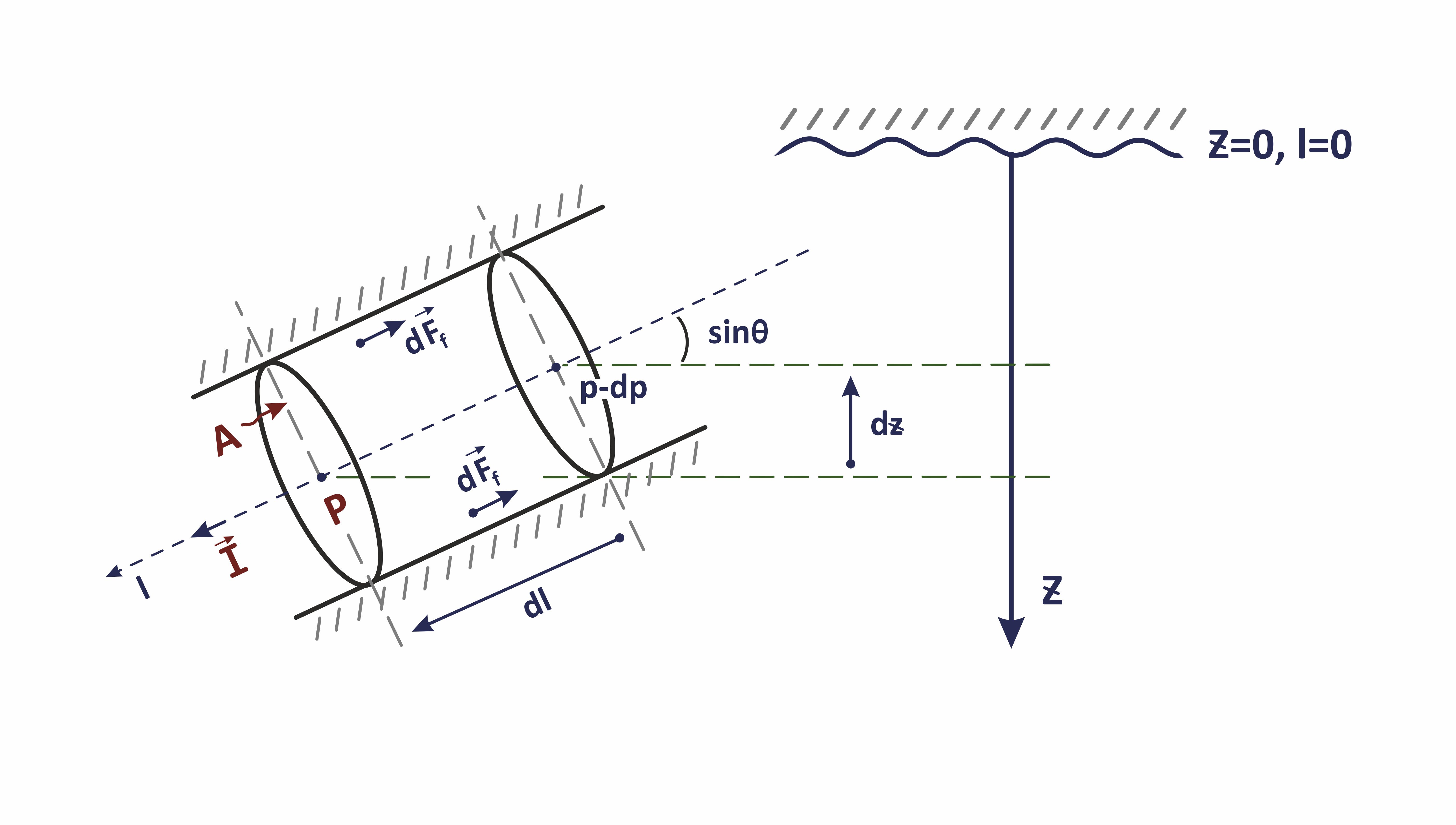
\frac{\partial T}{\partial lt} = 0, -\quad \frac{dp\partial P}{dl} + \rho_m \, g \, \sin \theta -\partial t} = 0, \quad \frac{\partial fu_m }{\, \rho_m \, u_m^2 \, }{2 d}partial t} = 0 |
The model is defined by the following set of 1D equations:
| LaTeX Math Block | ||||
|---|---|---|---|---|
| ||||
\sum_\alphaA(l) \rho_m u_m = \rho_\alpha \ c{sm} q_{p \alpha}s} = \rm const |
| LaTeX Math Block | ||||
|---|---|---|---|---|
| ||||
\frac{dp}{dl} = - \rho_m u_mu_\alpha \frac{\partial Tu_m}{\partial l} \ = + \rho_m \, g \, \frac{1}{A} cos \theta + \frac{ \sumf_m \alpha, \rho_m \, u_m^2 \, }{2 d} |
| LaTeX Math Block | ||||
|---|---|---|---|---|
| ||||
\sum_\alpha \big( \rho_\alpha \, c_{p \, \alpha} T_\alpha \big) \ q_m \ \frac{\partial q_\alphaT}{\partial l} |
It carries the original reservoir temperature with heating/cooling effect from reservoir-flow throttling and well-reservoir contact throttling:
| LaTeX Math Block | ||||
|---|---|---|---|---|
| ||||
T_\alpha = T_r + \epsilon \ = \ \sum_\alpha \rho_\,alpha \delta P =c_{p \alpha} T_r +\alpha \epsilon_\alpha \, (P_e - P_{wf}) |
where
| LaTeX Math Inline | ||
|---|---|---|
|
| LaTeX Math Inline | ||
|---|---|---|
|
time and space corrdinates ,
-axis is orientated towards the Earth centre, LaTeX Math Inline body z
define transversal plane to the LaTeX Math Inline body (x,y)
-axisLaTeX Math Inline body z
| LaTeX Math Inline | ||
|---|---|---|
|
measured depth along wellbore trajectory
| LaTeX Math Inline | ||
|---|---|---|
|
| LaTeX Math Inline | ||
|---|---|---|
|
| LaTeX Math Inline | ||
|---|---|---|
|
| LaTeX Math Inline | ||
|---|---|---|
|
| LaTeX Math Inline | ||
|---|---|---|
|
differential Joule–Thomson coefficient of
| LaTeX Math Inline | ||
|---|---|---|
|
| LaTeX Math Inline | ||
|---|---|---|
|
| LaTeX Math Inline | ||
|---|---|---|
|
differential adiabatic coefficient of
| LaTeX Math Inline | ||
|---|---|---|
|
| LaTeX Math Inline | ||
|---|---|---|
|
| LaTeX Math Inline | ||
|---|---|---|
|
Darci flow friction coefficient at fluid velocity
| LaTeX Math Inline | ||
|---|---|---|
|
| LaTeX Math Inline | ||
|---|---|---|
|
| LaTeX Math Inline | ||
|---|---|---|
|
| LaTeX Math Inline | ||
|---|---|---|
|
| LaTeX Math Inline | ||
|---|---|---|
|
cross-sectional area
| LaTeX Math Inline | ||
|---|---|---|
|
| LaTeX Math Inline | ||
|---|---|---|
|
volumetric flow rate
| LaTeX Math Inline | ||
|---|---|---|
|
| LaTeX Math Inline | ||
|---|---|---|
|
| LaTeX Math Inline | ||
|---|---|---|
|
| LaTeX Math Inline | ||
|---|---|---|
|
in-situ velocity of
| LaTeX Math Inline | ||
|---|---|---|
|
| LaTeX Math Inline | ||
|---|---|---|
|
gravitational acceleration constant
| LaTeX Math Inline | ||
|---|---|---|
|
| LaTeX Math Inline | ||
|---|---|---|
|
| LaTeX Math Inline | ||
|---|---|---|
|
| LaTeX Math Inline | ||
|---|---|---|
|
| LaTeX Math Inline | ||
|---|---|---|
|
effective thermal conductivity of the rocks with account for multiphase fluid saturation
| LaTeX Math Inline | ||
|---|---|---|
|
| LaTeX Math Inline | ||
|---|---|---|
|
| LaTeX Math Inline | ||
|---|---|---|
|
kinematic viscosity of
| LaTeX Math Inline | ||
|---|---|---|
|
| LaTeX Math Inline | ||
|---|---|---|
|
thermal conductivity of
-phase fluidLaTeX Math Inline body \alpha
| LaTeX Math Inline | ||
|---|---|---|
|
dynamic viscosity of
| LaTeX Math Inline | ||
|---|---|---|
|
| LaTeX Math Inline | ||
|---|---|---|
|
rock matrix mass density
| LaTeX Math Inline | ||
|---|---|---|
|
specific isobaric heat capacity of
| LaTeX Math Inline | ||
|---|---|---|
|
| LaTeX Math Inline | ||
|---|---|---|
|
specific isobaric heat capacity of the rock matrix
frac{\partial q_\alpha}{\partial l} |
The right side of equation
| LaTeX Math Block Reference | ||
|---|---|---|
|
| LaTeX Math Inline | ||
|---|---|---|
|
| LaTeX Math Block | ||||
|---|---|---|---|---|
| ||||
T_\alpha = T_r + \epsilon_\alpha \, \delta p = T_r + \epsilon_\alpha \, (p_e - p) |
The discrete computational scheme for
| LaTeX Math Block Reference | ||
|---|---|---|
|
| LaTeX Math Block | ||||
|---|---|---|---|---|
| ||||
\bigg( \sum_\alpha \rho_\alpha^{k-1} \ c_{p \alpha}^{k-1} \ q_\alpha^{k-1} \bigg) T^{k-1} - \bigg( \sum_\alpha \rho_\alpha^k \ c_{p \alpha}^k \ q_\alpha^k \bigg) T^k
= \sum_\alpha \rho_\alpha^k \ c_{p \alpha}^k \ (q_\alpha^{k-1} - q_\alpha^k) \, (T_r^k + \epsilon_\alpha^k \delta p^k ) |
where
| LaTeX Math Inline | ||
|---|---|---|
|
| LaTeX Math Inline | ||
|---|---|---|
|
| LaTeX Math Inline | ||
|---|---|---|
|
| LaTeX Math Inline | ||
|---|---|---|
|
| LaTeX Math Inline | ||
|---|---|---|
|
| LaTeX Math Inline | ||
|---|---|---|
|
| LaTeX Math Inline | ||
|---|---|---|
|
The
| LaTeX Math Inline | ||
|---|---|---|
|
| LaTeX Math Inline | ||
|---|---|---|
|
| LaTeX Math Inline | ||
|---|---|---|
|
If the flowrate is not vanishing during the stationary lift (
| LaTeX Math Inline | ||
|---|---|---|
|
| LaTeX Math Inline | ||
|---|---|---|
|
| LaTeX Math Inline | ||
|---|---|---|
|
| LaTeX Math Block | ||||
|---|---|---|---|---|
| ||||
T^{k-1} = \frac{\bigg( \sum_\alpha \rho_\alpha^k \ c_{p \alpha}^k \ q_\alpha^k \bigg) T^k + \sum_\alpha \rho_\alpha^k \ c_{p \alpha}^k \ (q_\alpha^{k-1} - q_\alpha^k) \, (T_r^k + \epsilon_\alpha^k \delta p^k )}{\bigg( \sum_\alpha \rho_\alpha^{k-1} \ c_{p \alpha}^{k-1} \ q_\alpha^{k-1} \bigg) }
|
Slippage Model
The multiphase slippage wellbore flow model assumes that fluid is at hydrodynamic and thermodynamic equilibrium and there is a slip between phases so that phases may be moving with different flow speeds
| LaTeX Math Inline | ||
|---|---|---|
|
The model is defined by the following set of 1D equations:
| LaTeX Math Block | ||||
|---|---|---|---|---|
| ||||
A(l) |
The discrete computational scheme for
| LaTeX Math Block Reference | ||
|---|---|---|
|
| LaTeX Math Block | ||||
|---|---|---|---|---|
| ||||
\bigg( \sum_\alpha \rho_\alpha^{k-1} \ c_{p \alpha}^{k-1} \ q_\alpha^{k-1} \bigg) T^{k-1} - \bigg( alpha u_\alpha = \sum_\alpha \rho_{s\alpha} q_{s\alpha} = \rm const |
| LaTeX Math Block | ||||
|---|---|---|---|---|
| ||||
\sum_\alpha \rho_\alpha^kalpha u_\alpha c_{p \frac{\partial u_\alpha}^k {\ q_\alpha^k \bigg) T^k partial l} = - \sum_\alphafrac{dp}{dl} + \rho_m \alpha^k, g \ c_{p, \cos \alpha}^ktheta \+ (q_\alpha^frac{k-1} - q_\alpha^k) f_m \, (T\rho_r^km +\, \epsilonu_\alpha^km^2 \delta, p^k ) |
where
| LaTeX Math Inline | ||
|---|---|---|
|
| LaTeX Math Inline | ||
|---|---|---|
|
| LaTeX Math Inline | ||
|---|---|---|
|
| LaTeX Math Inline | ||
|---|---|---|
|
| LaTeX Math Inline | ||
|---|---|---|
|
| LaTeX Math Inline | ||
|---|---|---|
|
| LaTeX Math Inline | ||
|---|---|---|
|
The
| LaTeX Math Inline | ||
|---|---|---|
|
| LaTeX Math Inline | ||
|---|---|---|
|
| LaTeX Math Inline | ||
|---|---|---|
|
If the flowrate is not vanishing during the stationary lift (
| LaTeX Math Inline | ||
|---|---|---|
|
| LaTeX Math Inline | ||
|---|---|---|
|
| LaTeX Math Inline | ||
|---|---|---|
|
| LaTeX Math Block | ||||
|---|---|---|---|---|
| ||||
T^{k-1} = \frac{\bigg( \sum_\alpha \rho_\alpha^k \ c_{p \alpha}^k \ q_\alpha^k \bigg) T^k + \sum_\alpha \rho_\alpha^k \ c_{p \alpha}^k \ (q_\alpha^{k-1} - q_\alpha^k) \, (T_r^k + \epsilon_\alpha^k \delta p^k )}{\bigg( \sum_\alpha \rho_\alpha^{k-1} \ c_{p \alpha}^{k-1} \ q_\alpha^{k-1} \bigg) }
|
| title | Derivation |
|---|
| LaTeX Math Block | ||||
|---|---|---|---|---|
| ||||
(\rho \,c_{pt})_p \frac{\partial T}{\partial t}

-  \sum_{a = \{w,o,g \}} \rho_\alpha \ c_{p \alpha} \ \eta_{s \alpha} \ \frac{\partial P_\alpha}{\partial t}

+  \sum_{a = \{w,o,g \}} \rho_\alpha \ c_{p \alpha} \ u_\alpha \frac{\partial T}{\partial l}
\ = \ \frac{\delta E_H}{ \delta V \delta t} |
Equation
| LaTeX Math Block Reference | ||
|---|---|---|
|
The term
| LaTeX Math Inline | ||
|---|---|---|
|
| LaTeX Math Inline | ||
|---|---|---|
|
The multiphase wellbore flow in hydrodynamic and thermodynamic equilibrium is defined by the following set of 1D equations:
| LaTeX Math Block | ||||
|---|---|---|---|---|
| ||||
\frac{\partial (\rho_m A)}{\partial t} + \frac{\partial}{\partial l} \bigg( A \, \sum_\alpha \rho_\alpha \, u_\alpha \bigg) = 0 |
| LaTeX Math Block | ||||
|---|---|---|---|---|
| ||||
\sum_\alpha \rho_\alpha \bigg[ \frac{\partial u_\alpha}{\partial t} + u_\alpha \frac{\partial u_\alpha}{\partial l} - \nu_\alpha \Delta u_\alpha\bigg] = - \frac{dp}{dl} + \rho_m \, g \, \sin \theta - \frac{ f_m \, \rho_m \, u_m^2 \, }{2 d} |
| LaTeX Math Block | ||||
|---|---|---|---|---|
| ||||
(\rho \,c_p)_m \frac{\partial T}{\partial t}

- \bigg( \sum_\alpha \rho_\alpha \ c_{p \alpha} \ \eta_{s \alpha}\bigg) \ \frac{\partial p}{\partial t}

+ \bigg( \sum_\alpha \rho_\alpha \ c_{p \alpha} \ u_\alpha \bigg) \frac{\partial T}{\partial l}
\ = \ \frac{1}{A} \ \sum_\alpha \rho_\alpha \ c_{p \alpha} T_\alpha \frac{\partial q_\alpha}{\partial l} |
Equations
| LaTeX Math Block Reference | ||
|---|---|---|
|
| LaTeX Math Block Reference | ||
|---|---|---|
|
| LaTeX Math Inline | ||
|---|---|---|
|
| LaTeX Math Inline | ||
|---|---|---|
|
| LaTeX Math Inline | ||
|---|---|---|
|
The model is set in 1D-model with
| LaTeX Math Inline | ||
|---|---|---|
|
| LaTeX Math Inline | ||
|---|---|---|
|
The disambiguation of the properties in the above equation is brought in The list of dynamic flow properties and model parameters.
Equation
| LaTeX Math Block Reference | ||
|---|---|---|
|
| LaTeX Math Inline | ||
|---|---|---|
|
Equation
| LaTeX Math Block Reference | ||
|---|---|---|
|
| LaTeX Math Inline | ||
|---|---|---|
|
| LaTeX Math Inline | ||
|---|---|---|
|
| LaTeX Math Inline | ||
|---|---|---|
|
The term
| LaTeX Math Inline | ||
|---|---|---|
|
This usually takes effect in the wellbore during the first minutes or hours after changing the well flow regime (as a consequence of choke/pump operation).
The term
| LaTeX Math Inline | ||
|---|---|---|
|
| LaTeX Math Block | ||||
|---|---|---|---|---|
| ||||
(\rho \,c_p)_m = \sum_\alpha \rho_\alpha c_\alpha s_\alpha |
Stationary wellbore flow is defined as the flow with constant pressure and temperature:
| LaTeX Math Inline | ||
|---|---|---|
|
| LaTeX Math Inline | ||
|---|---|---|
|
This happens during the long-term (usually hours & days & weeks) production/injection or long-term (usually hours & days & weeks) shut-in.
| LaTeX Math Block | ||||
|---|---|---|---|---|
| ||||
(\rho \,c_{pt})_p \frac{\partial T}{\partial t}

- \ \phi \sum_{a = \{w,o,g \}} \rho_\alpha \ c_{p \alpha} \ \eta_{s \alpha} \ \frac{\partial P_\alpha}{\partial t}

+ \bigg( \sum_{a = \{w,o,g \}} \rho_\alpha \ c_{p \alpha} \ \epsilon_\alpha \ \mathbf{u}_\alpha \bigg)  \nabla P

+ \bigg( \sum_{a = \{w,o,g \}} \rho_\alpha \ c_{p \alpha} \ \mathbf{u}_\alpha \bigg) \  \nabla T

- \nabla (\lambda_t \nabla T) = \frac{\delta E_H}{ \delta V \delta t} |
The wellbore fluid velocity
| LaTeX Math Inline | ||
|---|---|---|
|
| LaTeX Math Inline | ||
|---|---|---|
|
| LaTeX Math Inline | ||
|---|---|---|
|
| LaTeX Math Block | ||||
|---|---|---|---|---|
| ||||
u_\alpha = \frac{q_\alpha}{\pi r_f^2} |
so that
| LaTeX Math Block | ||||
|---|---|---|---|---|
| ||||
\bigg( \sum_{a = \{w,o,g \}} \rho_\alpha \ c_{p \alpha} \ \mathbf{u}_\alpha \bigg) \  \nabla T
= \frac{\delta E_H}{ \delta V \delta t} |
References
Beggs, H. D. and Brill, J. P.: "A Study of Two-Phase Flow in Inclined Pipes," J. Pet. Tech., May (1973), 607-617}{2 d} |
| LaTeX Math Block | ||||
|---|---|---|---|---|
| ||||
\sum_\alpha \rho_\alpha \ c_{p \alpha} \ u_\alpha \frac{\partial T}{\partial l}
\ = \ \frac{1}{A} \ \sum_\alpha \rho_\alpha \ c_{p \alpha} T_\alpha \frac{\partial q_\alpha}{\partial l} |
It carries the original reservoir temperature with heating/cooling effect from reservoir-flow throttling and well-reservoir contact throttling:
| LaTeX Math Block | ||||
|---|---|---|---|---|
| ||||
T_\alpha = T_r + \epsilon_\alpha \, \delta P = T_r + \epsilon_\alpha \, (P_e - P_{wf}) |
see Nomenclature below.
References
| Anchor | ||||
|---|---|---|---|---|
|
Nomenclature
| position vector at which the flow equations are set | ||||||||||||||||||||||
| time and space corrdinates ,
| ||||||||||||||||||||||
| measured depth along wellbore trajectory
| ||||||||||||||||||||||
| indicates a mixture of fluid phases | ||||||||||||||||||||||
| water, oil, gas phase indicator |
| differential Joule–Thomson coefficient of
| ||||||||||||||||||||
| pressure at separator |
| differential adiabatic coefficient of
| ||||||||||||||||||||
| temperature at separator |
| Darcy friction factor at fluid velocity
| ||||||||||||||||||||
| wellbore fluid pressure |
| cross-sectional average pipe flow diameter | ||||||||||||||||||||
| wellbore fluid temperature |
| cross-sectional area
| ||||||||||||||||||||
| volumetric flow rate
|
| wellbore trajectory inclination to horizon | ||||||||||||||||||||
| in-situ velocity of
|
| gravitational acceleration constant | ||||||||||||||||||||
|
|
| effective thermal conductivity of the rocks with account for multiphase fluid saturation | ||||||||||||||||||||
| cross-sectional average fluid density |
| rock matrix thermal conductivity | ||||||||||||||||||||
| kinematic viscosity of
|
| thermal conductivity of | ||||||||||||||||||||
| dynamic viscosity of
|
| rock matrix mass density | ||||||||||||||||||||
| specific isobaric heat capacity of
|
| specific isobaric heat capacity of the rock matrix | ||||||||||||||||||||