Definition
...
Mathematical Model
...
Motivation
Assume the well is producing
of water, of oil and ...
| LaTeX Math Block |
|---|
|
(\rho \,c_{pt})_p \frac{\partial T}{\partial t}

-  \sum_{a = \{w,o,g \}} \rho_\alpha \ c_{p \alpha} \ \eta_{s \alpha} \ \frac{\partial P_\alpha}{\partial t}

+  \sum_{a = \{w,o,g \}} \rho_\alpha \ c_{p \alpha} \ u_\alpha \frac{\partial T}{\partial l}
\ = \ \frac{\delta E_H}{ \delta V \delta t} |
The disambiguation of the properties in the above equation is brought in The list of dynamic flow properties and model parameters.
Equations ??? define the continuity of the fluid components flow or equivalently represent the mass conservation of each mass component
| LaTeX Math Inline |
|---|
| body | \{ m_W, \ m_O, \ m_G \} |
|---|
|
during its transportation in space. Equations ??? define the motion dynamics of each phase, represented as linear correlation between phase flow speed
and partial pressure gradient of this phase .Equation
| LaTeX Math Block Reference |
|---|
|
defines the heat flow continuity or equivalently represents heat conservation due to heat conduction and convection with account for adiabatic and Joule–Thomson throttling effect.The term
| LaTeX Math Inline |
|---|
| body | \frac{\delta E_H}{ \delta V \delta t} |
|---|
|
defines the speed of change of heat energy volumetric density due to the inflow from formation into the wellbore....
| LaTeX Math Inline |
|---|
| body | \sum_{a = \{w,o,g \}} \rho_\alpha \ c_{p \alpha} \ u_\alpha \frac{\partial T}{\partial l} |
|---|
|
...
The term
| LaTeX Math Inline |
|---|
| body | \sum_{a = \{w,o,g \}} \rho_\alpha \ c_{p \alpha} \ \eta_{s \alpha} \ \frac{\partial P_\alpha}{\partial t} |
|---|
|
represents the heating/cooling effect of the fast adiabatic pressure change. This usually takes effect in and around the wellbore during the first minutes or hours after changing the well flow regime (as a consequence of choke/pump operation). This effect is absent in stationary flow and negligible during the quasi-stationary flow and usually not modeled in conventional monthly-based flow simulations. Stationary Flow Model
Stationary wellbore flow is defined as the flow with constant pressure and temperature:
| LaTeX Math Inline |
|---|
| body | \frac{\partial T}{\partial t} = 0 |
|---|
|
and | LaTeX Math Inline |
|---|
| body | \frac{\partial P_\alpha}{\partial t} = 0 |
|---|
|
.This happens during the long-term (usually hours & days & weeks) production/injection or long-term (usually hours & days & weeks) shut-in.
The temperature dynamic equation
| LaTeX Math Block Reference |
|---|
|
is going to be:| LaTeX Math Block |
|---|
|
\bigg( \sum_{a = \{w,o,g \}} \rho_\alpha \ c_{p \alpha} \ \mathbf{u}_\alpha \bigg) \  \nabla T
= \frac{\delta E_H}{ \delta V \delta t} |
and its discrete computational scheme will be:
| LaTeX Math Block |
|---|
|
\bigg( \sum_{a = \{w,o,g \}} \rho_\alpha^{k-1} \ c_{p \alpha}^{k-1} \ q_\alpha^{k-1} \bigg) T^{k-1} - \bigg( \sum_{a = \{w,o,g \}} \rho_\alpha^k \ c_{p \alpha}^k \ q_\alpha^k \bigg) T^k
= \sum_{a = \{w,o,g \}} \rho_\alpha^k \ c_{p \alpha}^k \ (q_\alpha^{k-1} - q_\alpha^k) \, (T_r^k + \epsilon_\alpha^k \delta p^k ) |
where
| LaTeX Math Inline |
|---|
| body | \delta p^k = p_e^k - p_{wf}^k |
|---|
|
is drawdown, – formation pressure in th grid layer, – bottom-hole pressure across th grid layer, – remote reservoir temperature of th grid layer.The
axis is pointing downward along hole with th grid layer sitting above the th grid layer.If the flowrate is not vanishing during the stationary lift (
| LaTeX Math Inline |
|---|
| body | \sum_{a = \{w,o,g \}} |q_\alpha^{k-1}| > 0 |
|---|
|
) then can be calculated iteratively from previous values of the wellbore temperature as:| LaTeX Math Block |
|---|
|
T^{k-1} = \frac{\bigg( \sum_{a = \{w,o,g \}} \rho_\alpha^k \ c_{p \alpha}^k \ q_\alpha^k \bigg) T^k + \sum_{a = \{w,o,g \}} \rho_\alpha^k \ c_{p \alpha}^k \ (q_\alpha^{k-1} - q_\alpha^k) \, (T_r^k + \epsilon_\alpha^k \delta p^k )}{\bigg( \sum_{a = \{w,o,g \}} \rho_\alpha^{k-1} \ c_{p \alpha}^{k-1} \ q_\alpha^{k-1} \bigg) } |
...
| LaTeX Math Block |
|---|
|
(\rho \,c_{pt})_p \frac{\partial T}{\partial t}

- \ \phi \sum_{a = \{w,o,g \}} \rho_\alpha \ c_{p \alpha} \ \eta_{s \alpha} \ \frac{\partial P_\alpha}{\partial t}

+ \bigg( \sum_{a = \{w,o,g \}} \rho_\alpha \ c_{p \alpha} \ \epsilon_\alpha \ \mathbf{u}_\alpha \bigg)  \nabla P

+ \bigg( \sum_{a = \{w,o,g \}} \rho_\alpha \ c_{p \alpha} \ \mathbf{u}_\alpha \bigg) \  \nabla T

- \nabla (\lambda_t \nabla T) = \frac{\delta E_H}{ \delta V \delta t} |
The wellbore fluid velocity
can be expressed thorugh the volumetric flow profile and tubing/casing cross-section area as:| LaTeX Math Block |
|---|
|
u_\alpha = \frac{q_\alpha}{\pi r_f^2} |
so that
| LaTeX Math Block |
|---|
|
\bigg( \sum_{a = \{w,o,g \}} \rho_\alpha \ c_{p \alpha} \ \mathbf{u}_\alpha \bigg) \  \nabla T
= \frac{\delta E_H}{ \delta V \delta t} |
References
Beggs, H. D. and Brill, J. P.: "A Study of Two-Phase Flow in Inclined Pipes," J. Pet. Tech., May (1973), 607-617
...
...
Физическая картина течения флюида
В зависимости от компонентного состава поток жидкости может классифицироваться как однофазный или многофазный. Первый характерен для газои водонагнетательных скважин, недавно введенных в эксплуатацию добывающих нефтяных и газовых скважин, а также сильно обводненных добывающих скважин, в то время как второй тип встречается, как правило, в большинстве скважин, находящихся в эксплуатации в течение длительного времени. В общем случае, анализ многофазного потока может быть произведен для четырехфазного потока, включающего следующие фазы:
- Пластовая вода;
- Нагнетаемая вода;
...
- Турбулентный поток реализуется при высоких значениях числа Рейнольдса, при этом преобладают инерционные силы, что приводит к образованию хаотических завихрений и прочих нестабильностей потока. Значение числа Рейнольдса, как правило, выше 2300.
...
- Ламинарный поток имеет место при низких значениях числа Рейнольдса, при которых вязкие силы являются преобладающими, и характеризуется плавным и стабильным движением жидкости. Значение числа Рейнольдса, как правило, не превышает 2300.
...
of gas as measured daily at separator with pressure and temperature . While going down to depth
along the hole the wellbore pressure will be growing due to gravity of fluid column and friction losses emerging from fluid contact with inner pipe walls . Wellbore temperature
will be also varying due to heat exchange with surrounding rocks.The volume shares
| LaTeX Math Inline |
|---|
| body | \{ s_w(l), \, s_o(l), \, s_g(l) \} |
|---|
|
, occupied by different phases will be varying along hole due to along-hole pressure-temperature variation, phase segregation and phase slippage.It is now possible to simulate the stationary multiphase wellbore flow and link the surface flow conditions (pressure, temperature and rates) to downhole flow conditions at any depth.
| Expand |
|---|
|
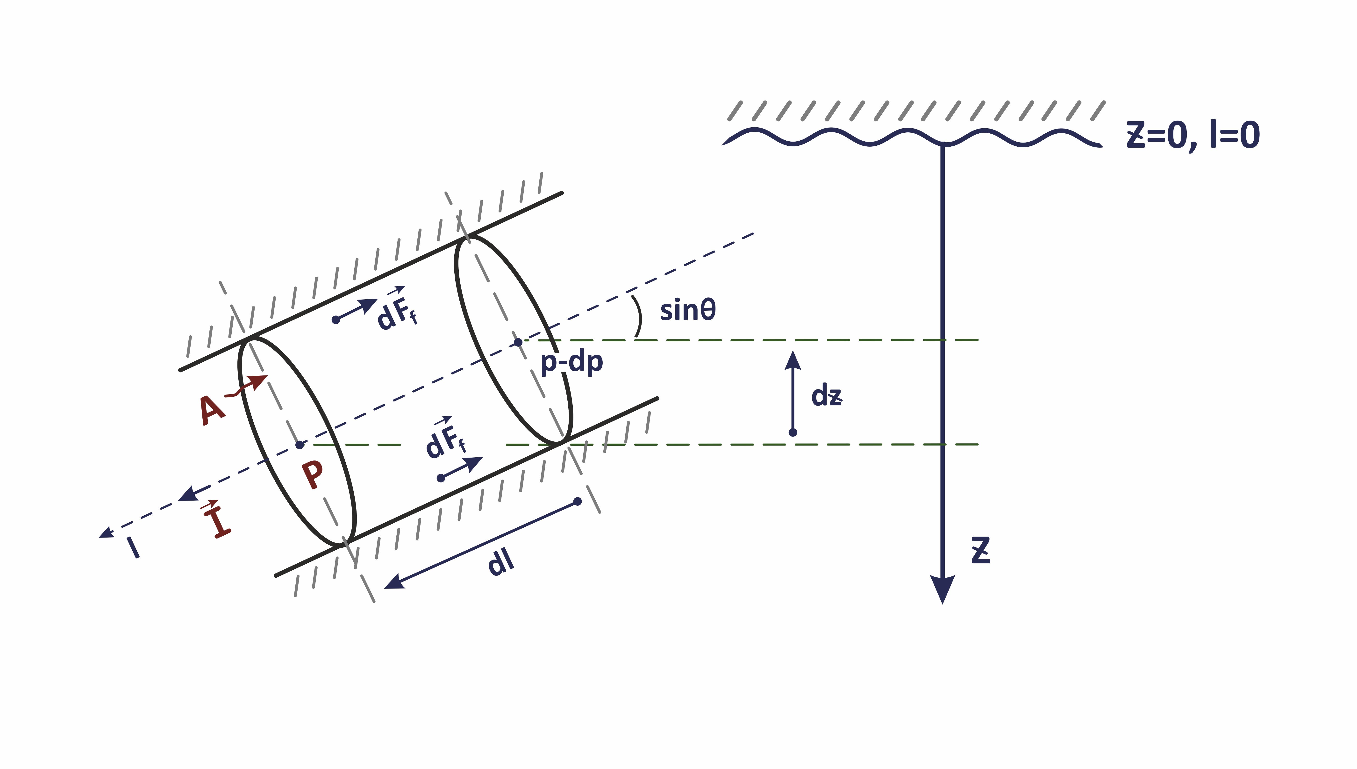 Image Added Image Added
| | Fig. 1. Wellbore Flow Model geometry |
|
The most adequate and practical model can be built for a stationary fluid flow at hydrodynamic and thermodynamic equilibrium.
If flow is changing slowly over time the same solutions can be used with inputs as time functions which is called quasi-stationary flow conditions.
This model finds important applications in industry.
If well production has been changed abruptly (for example opening or closing the flow) there will be a transition period towards the new quasi-stationary flow conditions (usually minutes or few hours).
The transition period for pressure and temperature is different and wellbore temperature takes much longer time to stabilize than pressure.
Unlike single-phase flow (Wellbore Water Flow and Wellbore Gas Flow) the complexity of the multiphase flow during transition is so high and unstable that building a simple mathematical model does not make a practical sense.
Definition
Mathematical model of Multiphase Wellbore Flow predicts the temperature, pressure and flow speed distribution along the wellbore trajectory with account for:
- tubing head pressure which is controled by gathering system or injection pump
- wellbore design (pipe diameters, pipe materials and inter-pipe annular fillings)
- fluid friction with tubing /casing walls
- interfacial phase slippage
- heat exchange between wellbore fluid and surrounding rocks via complex well design
Consider a 3-phase water-oil-gas flow:
| LaTeX Math Inline |
|---|
| body | \alpha = \{ w, \, o, \, g \} |
|---|
|
.
The
-phase volumetric flow fraction ( also called phase cut or input hold-up or no-slip hold-up ) is defined as:| LaTeX Math Block |
|---|
|
\gamma_\alpha = \frac{q_\alpha}{q_t} |
where
– volumetric flow rate of -phase and is the total volumetric fluid production rate:| LaTeX Math Block |
|---|
|
q_t = \sum_\alpha q_\alpha = q_w + q_o + g_g |
In multiphase wellbore flow each phase occupies its own area
of the total cross-sectional area of the lifting pipe. This area can be connected into a single piece of cross-sectional area (like in case of slug or annular flow) or dispersed into a number of connected spots (like in case of bubbly flow).
A share of total pipe cross-section area occupied by moving
-phase is called an -phase in-situ hold-up and defined as: | LaTeX Math Block |
|---|
|
s_\alpha = \frac{A_\alpha}{A} |
so that a sum of all in-situ hold-ups is subject to natural constraint:
| LaTeX Math Block |
|---|
| anchor | s_norm |
|---|
| alignment | left |
|---|
|
\sum_\alpha s_\alpha = s_w + s_o + s_g = 1 |
When word hold-up is used alone it usually means in-situ hold-up and should not be confused with input hold-up or no-slip hold-up which should be better called volumetric flow fraction.
The actual average cross-sectional velocity of moving
-phase is called in-situ velocity and defined as:| LaTeX Math Block |
|---|
|
u_\alpha = \frac{q_\alpha}{A_\alpha} |
where
is the volumetric -phase flowrate through cross-sectional area .
The superficial velocity of
-phase is defined as the | LaTeX Math Block |
|---|
|
u_{s \alpha} = \frac{q_\alpha}{A}= s_\alpha \cdot u_\alpha |
The multiphase mixture velocity is defined as total flow volume normalized by the total cross-sectional area:
| LaTeX Math Block |
|---|
|
u_m = \frac{1}{A} \sum_\alpha q_\alpha = \sum_\alpha u_{s \alpha} = \sum_\alpha s_\alpha \cdot u_\alpha |
The difference between velocities of
-phase and -phase is called interfacial phase phase slippage:| LaTeX Math Block |
|---|
|
u_{\alpha_1 \alpha_2} = u_{\alpha_1} - u_{\alpha_2} |
The multiphase fluid density
is defined by exact formula:| LaTeX Math Block |
|---|
|
\rho_m = \sum_\alpha s_\alpha \rho_\alpha |
where
– density of -phase.
The two-phase gas-liquid model is defined in the following terms:
| LaTeX Math Block |
|---|
|
u_m = u_{s g} + u_{s l} = s_g u_g + (1-s_g) u_l |
The two-phase oil-water model is defined in the following terms:
| LaTeX Math Block |
|---|
|
u_m = u_{s o} + u_{s w} = s_o u_o + (1-s_o-s_g) u_w |
The 3-phase water-oil-gas model is usually built as a superposition of gas-liquid model and then oil-water model:
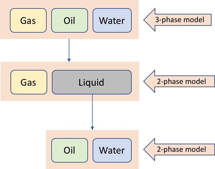 Image Added
Input & Output
| Input | Output |
|---|
| LaTeX Math Inline |
|---|
| body | p_s, \, T_s, \ \{ q_w, q_o, \, q_g \} |
|---|
|
as values at separator | | LaTeX Math Inline |
|---|
| body | p(l), \, T(l), \, \{ s_w(l), \, s_o(l), \, s_g(l) \}, \, \{ q_w(l), \, q_o(l), \, q_g(l) \} |
|---|
|
as logs along hole |
Application
| Activity |
| Input | Output |
|---|
| 1 | WPA – Well Performance Analysis | Optimizing the lift performance based on the IPR vs VLP models | | LaTeX Math Inline |
|---|
| body | p_s, \, T_s, \ \{ q_w, q_o, \, q_g \} |
|---|
|
as values at separator | | LaTeX Math Inline |
|---|
| body | p_{wf}(l = l_{datum}) |
|---|
|
as value at formation datum |
|---|
| 2 | DM – Dynamic Modelling | Relating production rates at separator to bottom-hole pressure with VLP | | LaTeX Math Inline |
|---|
| body | p_s, \, T_s, \ \{ q_w, q_o, \, q_g \} |
|---|
|
as values at separator | | LaTeX Math Inline |
|---|
| body | p_{wf}(l = l_{datum}) |
|---|
|
as value at formation datum |
|---|
| 3 | PRT – Pressure Testing | Adjust gauge pressure to formation datum | | LaTeX Math Inline |
|---|
| body | p_{wf}(l = l_{gauge}) |
|---|
|
as value at downhole gauge | | LaTeX Math Inline |
|---|
| body | p_{wf}(l = l_{datum}) |
|---|
|
as value at formation datum |
|---|
| 4 | PLT – Production Logging | Interpretation of production logs | | LaTeX Math Inline |
|---|
| body | \{ p(l), \, T(l), \, u_m(l), \, s_w(l), \, s_o(l), \, s_g(l) \} |
|---|
|
as logs along hole | | LaTeX Math Inline |
|---|
| body | \{ q_w(l), \, q_o(l), \, q_g(l) \} |
|---|
|
as logs along hole |
|---|
| 5 | RFP – Reservoir Flow Profiling | Interpretation of reservoir flow logs | | LaTeX Math Inline |
|---|
| body | \{ p(l), \, T(l), \, u_m(l), \, s_w(l), \, s_o(l), \, s_g(l) \} |
|---|
|
as logs along hole | | LaTeX Math Inline |
|---|
| body | \{ q_w(l), \, q_o(l), \, q_g(l) \} |
|---|
|
as logs along hole |
|---|
Mathematical Model
Homogeneous Model
The multiphase homogeneous wellbore flow model assumes that fluid is at stationary hydrodynamic and thermodynamic equilibrium and there is no slip between phases.
This means that all have the same temperature:
| LaTeX Math Block |
|---|
|
T_w = T_o = T_g = T |
same pressure:
| LaTeX Math Block |
|---|
|
P_w = P_o = P_g = T |
same velocity:
| LaTeX Math Block |
|---|
|
u_w = u_o = u_g = u_m |
and all dynamic fluid parameters are constant in time:
| LaTeX Math Block |
|---|
|
\frac{\partial T}{\partial t} = 0, \quad \frac{\partial P}{\partial t} = 0, \quad \frac{\partial u_m}{\partial t} = 0 |
The model is defined by the following set of 1D equations:
| LaTeX Math Block |
|---|
|
A(l) \rho_m u_m = \rho_{sm} q_{s} = \rm const |
| LaTeX Math Block |
|---|
|
\frac{dp}{dl} = - \rho_m u_m \frac{\partial u_m}{\partial l} + \rho_m \, g \, \cos \theta + \frac{ f_m \, \rho_m \, u_m^2 \, }{2 d} |
| LaTeX Math Block |
|---|
|
\sum_\alpha \big( \rho_\alpha \, c_{p \, \alpha}  \big) \ q_m \  \frac{\partial T}{\partial l}
\ = \ \sum_\alpha \rho_\alpha \ c_{p \alpha} T_\alpha \frac{\partial q_\alpha}{\partial l} |
The right side of equation
| LaTeX Math Block Reference |
|---|
|
represents the heat inflow resulting from the fluid flow from reservoir into a wellbore which carries the original reservoir temperature with heating/cooling effect from reservoir-flow throttling and well-reservoir contact throttling:| LaTeX Math Block |
|---|
|
T_\alpha = T_r + \epsilon_\alpha \, \delta p = T_r + \epsilon_\alpha \, (p_e - p) |
The discrete computational scheme for
| LaTeX Math Block Reference |
|---|
|
will be:| LaTeX Math Block |
|---|
|
\bigg( \sum_\alpha \rho_\alpha^{k-1} \ c_{p \alpha}^{k-1} \ q_\alpha^{k-1} \bigg) T^{k-1} - \bigg( \sum_\alpha \rho_\alpha^k \ c_{p \alpha}^k \ q_\alpha^k \bigg) T^k
= \sum_\alpha \rho_\alpha^k \ c_{p \alpha}^k \ (q_\alpha^{k-1} - q_\alpha^k) \, (T_r^k + \epsilon_\alpha^k \delta p^k ) |
where
| LaTeX Math Inline |
|---|
| body | \delta p^k = p_e^k - p_{wf}^k |
|---|
|
is drawdown, – formation pressure in -th grid layer, – bottom-hole pressure across -th grid layer, – remote reservoir temperature of -th grid layer.The
-axis is pointing downward along hole with -th grid layer sitting above the -th grid layer.If the flowrate is not vanishing during the stationary lift (
| LaTeX Math Inline |
|---|
| body | \sum_{a = \{w,o,g \}} |q_\alpha^{k-1}| > 0 |
|---|
|
) then can be calculated iteratively from previous values of the wellbore temperature as:
| LaTeX Math Block |
|---|
|
T^{k-1} = \frac{\bigg( \sum_\alpha \rho_\alpha^k \ c_{p \alpha}^k \ q_\alpha^k \bigg) T^k + \sum_\alpha \rho_\alpha^k \ c_{p \alpha}^k \ (q_\alpha^{k-1} - q_\alpha^k) \, (T_r^k + \epsilon_\alpha^k \delta p^k )}{\bigg( \sum_\alpha \rho_\alpha^{k-1} \ c_{p \alpha}^{k-1} \ q_\alpha^{k-1} \bigg) }
|
Slippage Model
The multiphase slippage wellbore flow model assumes that fluid is at hydrodynamic and thermodynamic equilibrium and there is a slip between phases so that phases may be moving with different flow speeds
| LaTeX Math Inline |
|---|
| body | u_w \neq u_o \neq u_g |
|---|
|
.The model is defined by the following set of 1D equations:
| LaTeX Math Block |
|---|
|
A(l) \sum_\alpha \rho_\alpha u_\alpha = \sum_\alpha \rho_{s\alpha} q_{s\alpha} = \rm const |
| LaTeX Math Block |
|---|
|
\sum_\alpha \rho_\alpha u_\alpha \frac{\partial u_\alpha}{\partial l} = - \frac{dp}{dl} + \rho_m \, g \, \cos \theta + \frac{ f_m \, \rho_m \, u_m^2 \, }{2 d} |
| LaTeX Math Block |
|---|
|
\sum_\alpha \rho_\alpha \ c_{p \alpha} \ u_\alpha \frac{\partial T}{\partial l}
\ = \ \frac{1}{A} \ \sum_\alpha \rho_\alpha \ c_{p \alpha} T_\alpha \frac{\partial q_\alpha}{\partial l} |
It carries the original reservoir temperature with heating/cooling effect from reservoir-flow throttling and well-reservoir contact throttling:
| LaTeX Math Block |
|---|
|
T_\alpha = T_r + \epsilon_\alpha \, \delta P = T_r + \epsilon_\alpha \, (P_e - P_{wf}) |
see Nomenclature below.
Nomenclature
| LaTeX Math Inline |
|---|
| body | \mathbf{r} = (x, \ y, \ z) |
|---|
|
| position vector at which the flow equations are set |
| time and space corrdinates , -axis is orientated towards the Earth centre, define transversal plane to the -axis |
| measured depth along wellbore trajectory | LaTeX Math Inline |
|---|
| body | dl^2 = dx^2 + dy^2 + dz^2 |
|---|
|
starting from tubing head | LaTeX Math Inline |
|---|
| body | l (x = x_0, \ y=y_0, \ z = z_{THP}) = 0 |
|---|
|
|
| indicates a mixture of fluid phases |
| water, oil, gas phase indicator | | LaTeX Math Inline |
|---|
| body | \epsilon_\alpha (p, T) |
|---|
|
| differential Joule–Thomson coefficient of -phase fluid |
| pressure at separator | | differential adiabatic coefficient of -phase fluid |
| temperature at separator | | |
| wellbore fluid pressure | | cross-sectional average pipe flow diameter |
| wellbore fluid temperature | | cross-sectional area | LaTeX Math Inline |
|---|
| body | A(l) = 0.25 \, \pi \, d^2(l) |
|---|
|
|
| LaTeX Math Inline |
|---|
| body | q_\alpha(t, l) = \frac{d V_\alpha}{dt} |
|---|
|
| volumetric flow rate -phase fluid at wellbore depth | | wellbore trajectory inclination to horizon |
| in-situ velocity of -phase fluid flow | |
...
Модель
Тип скважины по углу наклона
...
Режимы многофазного потока
...
Вертикальная или с незначительным углом
...
Горизонтальная или сильно наклонная (с большим зенитным углом)
...
Полумеханистическая модель, основанная на теории скорости дрейфа, с использованием эмпирически определенных параметров и соблюдением условия непрерывности между различными режимами течения. Применяется при объемных содержаниях газа свыше 0.06.
...
Эмпирическая модель, в которой скорость проскальзывания фаз определяется с использованием семейства кривых, представляющих зависимость скорости проскальзывания от разницы плотности фаз и удельного содержания тяжелой фазы α_w (влагосодержание). Данная модель не учитывает различия между гидрофильными (капельки нефти в воде) и гидрофобными (капельки воды в нефти) смесями.
...
Полуэмпирическая модель, основанная на данных экспериментального исследования и допущениях модели скорости дрейфа. Данная модель не учитывает различия между гидрофильными (капельки нефти в воде)
и гидрофобными (капельки воды в нефти) смесями.
...
Стенфордская модель скорости дрейфа («жидкость-жидкость»)
[4,5]
...
Тип скважины по углу наклона
...
Режимы многофазного потока
...
Полумеханистическая модель, основанная на теории скорости дрейфа, с использованием эмпирически определенных параметров и соблюдением условия непрерывности между различными режимами течения. Применяется при объемных содержаниях газа свыше 0,06.
Дебиты фаз
...
| Column |
|---|
|
| LaTeX Math Block |
|---|
| Q_w = \sigma_{bh} \ \xi_w \ u_w |
| LaTeX Math Block |
|---|
| Q_o = \sigma_{bh} \ \xi_o \ u_o |
| LaTeX Math Block |
|---|
| Q_g = \sigma_{bh} \ \xi_g \ u_g |
|
| Column |
|---|
|
| LaTeX Math Block |
|---|
| u_w = \sigma_{bh} \ \frac{\xi_w}{\mu_w} \frac{d P_{\delta}}{dh} |
| LaTeX Math Block |
|---|
| u_o = \sigma_{bh} \ \frac{\xi_o}{\mu_o} \frac{d P_{\delta}}{dh} |
| LaTeX Math Block |
|---|
| u_g = \sigma_{bh} \ \frac{\xi_g}{\mu_g} \frac{d P_{\delta}}{dh} |
|
...
Распределение давления
| LaTeX Math Block |
|---|
|
Q(h) = Q_w + Q_o + Q_g = \int_{\Gamma_h} \big( q_w(h) + q_o(h) + q_g(h) \big) \ dh |
| LaTeX Math Block |
|---|
|
Q(h) = \sigma_{bh}^2 \bigg( \frac{\xi_w^2}{\mu_w} + \frac{\xi_o^2}{\mu_o} + \frac{\xi_g^2}{\mu_g} \bigg)\frac{d P_{\delta}}{dh} |
откуда
| LaTeX Math Block |
|---|
|
P_{\delta}(t, \delta h) = \int_0^{\delta h} \frac{Q(h) \ dh}{\sigma_{bh}^2 \bigg( \frac{\xi_w^2}{\mu_w} + \frac{\xi_o^2}{\mu_o} + \frac{\xi_g^2}{\mu_g} \bigg)} |
...
The list of dynamic flow properties and model parameters
...
...
time and space corrdinates ,
-axis is orientated towards the Earth centre, define transversal plane to the -axis...
| LaTeX Math Inline |
|---|
| body | \mathbf{r} = (x, \ y, \ z) |
|---|
|
...
| LaTeX Math Inline |
|---|
| body | q_{mW} = \frac{d m_W}{dt} |
|---|
|
...
speed of water-component mass change in wellbore draining points
...
| LaTeX Math Inline |
|---|
| body | q_{mO} = \frac{d m_O}{dt} |
|---|
|
...
speed of oil-component mass change in wellbore draining points
...
| LaTeX Math Inline |
|---|
| body | q_{mG} = \frac{d m_G}{dt} |
|---|
|
...
speed of gas-component mass change in wellbore draining points
...
| LaTeX Math Inline |
|---|
| body | q_W = \frac{1}{\rho_W^{\LARGE \circ}} \frac{d m_W}{dt} = \frac{d V_{Ww}^{\LARGE \circ}}{dt} = \frac{1}{B_w} q_w |
|---|
|
...
| LaTeX Math Inline |
|---|
| body | q_O = \frac{1}{\rho_O^{\LARGE \circ}} \frac{d m_O}{dt} = \frac{d V_{Oo}^{\LARGE \circ}}{dt} + \frac{d V_{Og}^{\LARGE \circ}}{dt} = \frac{1}{B_o} q_o + \frac{R_v}{B_g} q_g |
|---|
|
...
| LaTeX Math Inline |
|---|
| body | q_G = \frac{1}{\rho_G^{\LARGE \circ}} \frac{d m_G}{dt} = \frac{d V_{Gg}^{\LARGE \circ}}{dt} + \frac{d V_{Go}^{\LARGE \circ}}{dt} = \frac{1}{B_g} q_g + \frac{R_s}{B_o} q_o |
|---|
|
...
| LaTeX Math Inline |
|---|
| body | q_w = \frac{d V_w}{dt} |
|---|
|
...
| LaTeX Math Inline |
|---|
| body | q_o = \frac{d V_o}{dt} |
|---|
|
...
| LaTeX Math Inline |
|---|
| body | q_g = \frac{d V_g}{dt} |
|---|
|
...
| LaTeX Math Inline |
|---|
| body | q^S_W =\frac{dV_{Ww}^S}{dt} |
|---|
|
...
| LaTeX Math Inline |
|---|
| body | q^S_O = \frac{d (V_{Oo}^S + V_{Og}^S )}{dt} |
|---|
|
...
| LaTeX Math Inline |
|---|
| body | q^S_G = \frac{d (V_{Gg}^S + V_{Go}^S )}{dt} |
|---|
|
...
| LaTeX Math Inline |
|---|
| body | q^S_L = q^S_W + q^S_O |
|---|
|
...
| LaTeX Math Inline |
|---|
| body | P_w = P_w (t, \vec r) |
|---|
|
...
| LaTeX Math Inline |
|---|
| body | P_o = P_o (t, \vec r) |
|---|
|
...
| LaTeX Math Inline |
|---|
| body | P_g = P_g (t, \vec r) |
|---|
|
...
| LaTeX Math Inline |
|---|
| body | \vec u_w = \vec u_w (t, \vec r) |
|---|
|
...
| LaTeX Math Inline |
|---|
| body | \vec u_o = \vec u_o (t, \vec r) |
|---|
|
...
| LaTeX Math Inline |
|---|
| body | \vec u_g = \vec u_g (t, \vec r) |
|---|
|
...
| LaTeX Math Inline |
|---|
| body | P_{cow} = P_{cow} (s_w) |
|---|
|
capillary pressure at the oil-water phase contact as function of water saturation
...
| LaTeX Math Inline |
|---|
| body | P_{cog} = P_{cog} (s_ g) |
|---|
|
...
| LaTeX Math Inline |
|---|
| body | k_{rw} = k_{rw}(s_w, \ s_g) |
|---|
|
...
relative formation permeability to water flow as function of water and gas saturation
...
| LaTeX Math Inline |
|---|
| body | k_{ro} = k_{ro}(s_w, \ s_g) |
|---|
|
...
| LaTeX Math Inline |
|---|
| body | k_{rg} = k_{rg}(s_w, \ s_g) |
|---|
|
...
...
...
| LaTeX Math Inline |
|---|
| body | \vec g = (0, \ 0, \ g) |
|---|
|
...
| gravitational acceleration constant |
|
...
...
-phase fluid density at pressure |
...
...
...
| effective thermal conductivity of the rocks with account for multiphase fluid saturation |
| cross-sectional average fluid density | |
...
| rock matrix thermal conductivity |
|
...
...
...
kinematic viscosity of -phase |
...
...
...
...
...
| thermal conductivity of -phase fluid |
...
...
...
...
...
dynamic viscosity of -phase fluid | |
...
...
...
| specific isobaric heat capacity of -phase fluid | |
...
differential Joule–Thomson coefficient of
-phase fluid...
specific isobaric heat capacity of the rock matrix |