Сomparative analysis between:
- the reservoir fluid deliverability (the ability of reservoir to produce or take-in the fluid) which is called Inflow Performance Relation (IPR)
and
- wellbore fluid deliverability (the ability of well to lift up or lift down the fluid) and which is called Lift Curves (LC) (also called Vertical Lift Performance (VLP) or Tubing Performance Relation (TPR) )
Definition
...
It is based on correlation between surface flowrate and bottomhole pressure flowrate
| LaTeX Math Inline | ||
|---|---|---|
|
| LaTeX Math Inline | ||
|---|---|---|
|
| LaTeX Math Inline | ||
|---|---|---|
|
| LaTeX Math Inline | ||
|---|---|---|
|
Application
...
- Setting up the optimal production targets
Generating WFP – Well Flow Performance tables as input for 3D simulations
Technology
- the required production or injection regime for each well upon the current formation pressure, reservoir saturation and production target specified by FDP
- Generating Lift Curves (LC) tables as input for Reservoir Flow Modelling (RFM)
Technology
...
Anchor
In practice, the flow rate flowrate targets are closely related to bottomhole pressure and associated limitations and require a specialised analysis to set up the optimal lifting (completion, pump, chocke) parameters.
This is primary domain of WFP analysis.
WFP is performed on stabilised wellbore and reservoir flow and does not cover transient behavior behaviour which is one of the primary subjects of Well Testing domain.
The wellbore flow is called stabilised if the delta pressure across wellbore is not changing over time.
The formation flow is called stabilised if the well productivity index is not changing over time.
It's important to remember the difference between constant rate formation flow and stabilised formation flow.
...
On the other hand, the constant rate formation flow may not represent a stabilised formation flow as the bottom-hole pressure and productivity index maybe still in transition after the last rate change.
The WFP methods are not applicable if the well flow is not stabilised even if the flow rate is maintained constant.
There are two special reservoir flow regimes which are both stabilised and maintain constant flow rate: steady state regime (SS) and pseudo-steady state regime (PSS).
...
The pseudo-steady state (PSS) regime is reached when the flow is stabilised with no pressure support at the external boundary.
...
As for formation and bottom-hole pressure in PSS they will be synchronously varying while in SS they will be staying constant.
The table below is summarizing the major differences between SS and PSS regimes.
...
| LaTeX Math Inline | ||
|---|---|---|
|
...
constant
...
constant
...
| LaTeX Math Inline | ||
|---|---|---|
|
...
constant
...
constant
...
Drawdown
...
| LaTeX Math Inline | ||
|---|---|---|
|
...
constant
...
constant
...
| LaTeX Math Inline | ||
|---|---|---|
|
...
constant
...
varying
...
| LaTeX Math Inline | ||
|---|---|---|
|
...
constant
...
varying
It's again important to avoid confusion between the termines stationary conditions (which mean that refered properties are not chaning in time) and stabilised flow conditions which may admit pressure and rate vraition.
In practice, the productivity index is usually not known at all times as there is no routine procedure to assess it.
It is usually accepted that a given formation takes the same time to stabilise the flow after any change in well flow conditions and the stabilisation time is assessed based on the well tests analysis.
Although, this is not strictly true and the flow stabilisation time depends on well-formation contact and reservoir property variation around a given well.
This is also compromised in multi-layer formations with cross-layer communication.
The conventional WFP – Well Performance Analysis is perfomed as the
| LaTeX Math Inline | ||
|---|---|---|
|
...
...
IPR –
...
| LaTeX Math Inline | ||
|---|---|---|
|
...
| LaTeX Math Inline | ||
|---|---|---|
|
...
| anchor | 1 |
|---|---|
| alignment | left |
...
...
which may be non-linear.
...
...
| LaTeX Math Inline | ||
|---|---|---|
|
...
| LaTeX Math Block | ||||
|---|---|---|---|---|
| ||||
J_s(q_{\rm liq}) = \frac{q_{\rm liq}}{p_R-p_{wf}} |
for oil producer with surface liquid production
| LaTeX Math Inline | ||
|---|---|---|
|
- ) – responsible for reservoir deliverability (see below)
- Lift Curves (LC) – responsible for well deliverability (see below )
| Anchor | ||||
|---|---|---|---|---|
|
The intersection of IPR and Lift Curves represent the Stabilised wellbore flow (see Fig. 1)
|
|
| Fig. 1. A sample case of stabilised wellbore flow represented by junction point of IPR and Lift Curves. | Fig. 2. The dead well scenario. |
Given a tubing head pressure
| LaTeX Math Inline | ||
|---|---|---|
|
|
|
| Fig. 3. A sample case of stabilised wellbore flow as function of formation pressure. | Fig. 4. A sample case of stabilised wellbore flow as function of production watercut |
|
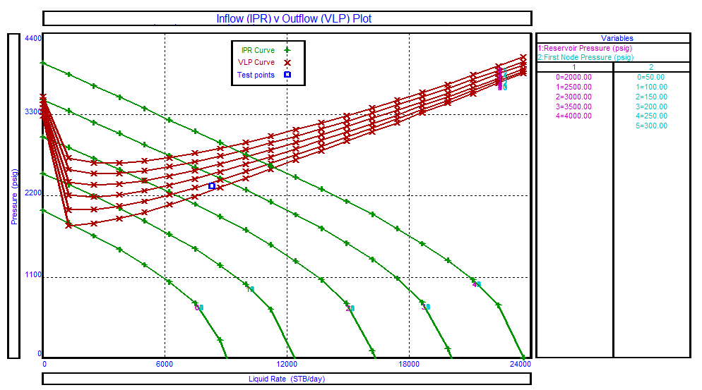
| Fig. 5. A bunch of IPRs at different formation pressures and Lift Curves at different THPs. |
Workflow
...
- Check the current production rate against the production target from FDP
- If the diffference is big enough to justify the cost of production optimization (see point 8 below) then proceed to the step 3 below
- Assess formation pressure based on well tests
- Simulate IPR / LC based on the current WOR/GOR
- Calculate the stabilized flow bottom-hole pressure
- Gather the current bottom-hole pressure
LaTeX Math Inline body p_{wf} - Check up the calculation aganst the actual
LaTeX Math Inline body p_{wf} - Recommend the production optimisation activities to adjust bottom-hole pressure
:LaTeX Math Inline body p_{wf} - adjusting the choke at surface
- adjusting the pump settings from surface
- changing the pump depth
- changing the tubing size
- changing the pump
- adjusting the choke at surface
The above workflow is very simplistic and assumes single-layer formation with no cross-flow complications.
In practise, the WFP analysis is often very tentative and production technologists spend some time experimenting with well regimes on well-by-well basis.
See Also
...
Petroleum Industry / Upstream / Production / Subsurface Production / Well & Reservoir Management
Subsurface E&P Disciplines / Production Technology
[ Inflow Performance Relation (IPR) ] [ Lift Curves (LC) ]
| Anchor | ||||
|---|---|---|---|---|
|
References
...
Joe Dunn Clegg, Petroleum Engineering Handbook, Vol. IV – Production Operations Engineering, SPE, 2007
Michael Golan, Curtis H. Whitson, Well Performance, Tapir Edition, 1996
William Lyons, Working Guide to Petroleum and Natural Gas production Engineering, Elsevier Inc., First Edition, 2010
Shlumberge, Well Performance Manual
...
| LaTeX Math Block | ||||
|---|---|---|---|---|
| ||||
J_s(q_g) = \frac{q_g}{p_R-p_{wf}} |
for gas producer
...
| LaTeX Math Block | ||||
|---|---|---|---|---|
| ||||
J_s(q_g) = \frac{q_g}{p_{wf}-p_R} |
for gas injector
...
| LaTeX Math Block | ||||
|---|---|---|---|---|
| ||||
J_s(q_w) = \frac{q_w}{p_R-p_{wf}} |
for water injector
where
...
| LaTeX Math Inline | ||
|---|---|---|
|
...
| LaTeX Math Inline | ||
|---|---|---|
|
...
field-average formation pressure withing the drainage area
| LaTeX Math Inline | ||
|---|---|---|
|
| LaTeX Math Inline | ||
|---|---|---|
|
Based on these notions the general WFP – Well Flow Performance can be wirtten in universal form:
| LaTeX Math Block | ||||
|---|---|---|---|---|
| ||||
p_{wf} = p_R - \frac{q}{J_s} |
providing that
| LaTeX Math Inline | ||
|---|---|---|
|
...
| LaTeX Math Inline | ||
|---|---|---|
|
...
| LaTeX Math Inline | ||
|---|---|---|
|
...
| LaTeX Math Inline | ||
|---|---|---|
|
...
| LaTeX Math Inline | ||
|---|---|---|
|
...
| LaTeX Math Inline | ||
|---|---|---|
|
...
For a single layer formation with low-compressibility fluid (like water) the PI does not depend on drwadown (or flowrate)
| LaTeX Math Inline | ||
|---|---|---|
|
...

...
This is a typical WFP – Well Flow Performance plot for water supply wells, water injectors and oil producers above bubble point.
The PI can be estimated using the Darcy equation:
| LaTeX Math Block | ||||
|---|---|---|---|---|
| ||||
J_s = \frac{2 \pi \sigma}{ \ln \frac{r_e}{r_w} + \epsilon+ S} |
where
| LaTeX Math Inline | ||
|---|---|---|
|
| LaTeX Math Block Reference | ||||
|---|---|---|---|---|
|
| LaTeX Math Inline | ||
|---|---|---|
|
| LaTeX Math Inline | ||
|---|---|---|
|
For gas wells, condensate producers, light-oil producers, and oil producers below bubble point
| LaTeX Math Inline | ||
|---|---|---|
|
It can be interpreted as deterioration of near-reservoir zone permeability with fluid velocity is growing.
...

...
Fig.2. WFP – Well Flow Performance for compressible fluid production (gas, light oil, saturated oil)
In general case of saturated oil, the PI
| LaTeX Math Inline | ||
|---|---|---|
|
| LaTeX Math Inline | ||
|---|---|---|
|
| LaTeX Math Inline | ||
|---|---|---|
|
But when field-average formation pressure is above bubble-point
| LaTeX Math Inline | ||
|---|---|---|
|
...
| title | Important Note |
|---|
Despite of terminological similarity there is a big difference in the way WFP and Well Testing deal with formation pressure and flowrates which results in a difference in productivity index definition and corresponding analysis.
This difference is summarized in the table below:
...
| LaTeX Math Inline | ||
|---|---|---|
|
field-average pressure within the drainage area
| LaTeX Math Inline | ||
|---|---|---|
|
...
| LaTeX Math Inline | ||
|---|---|---|
|
average pressure value at boudary of the drainage area
| LaTeX Math Inline | ||
|---|---|---|
|
...
| LaTeX Math Inline | ||
|---|---|---|
|
...
surface liquid rate
| LaTeX Math Inline | ||
|---|---|---|
|
...
| LaTeX Math Inline | ||
|---|---|---|
|
...
total flowrate at sandface
| LaTeX Math Inline | ||
|---|---|---|
|
...
| LaTeX Math Inline | ||
|---|---|---|
|
...
| LaTeX Math Inline | ||
|---|---|---|
|
| LaTeX Math Inline | ||
|---|---|---|
|
| LaTeX Math Inline | ||
|---|---|---|
|
...
| LaTeX Math Inline | ||
|---|---|---|
|
...
total multiphase proudcivity index
| LaTeX Math Inline | ||
|---|---|---|
|
...
VLP – Vertical Lift Performance
VLP – Vertical Lift Performance also called Outflow Performance Relation or Tubing Performance Relation represents the relation between the bottom-hole pressure
| LaTeX Math Inline | ||
|---|---|---|
|
| LaTeX Math Inline | ||
|---|---|---|
|
| LaTeX Math Block | ||||
|---|---|---|---|---|
| ||||
p_{wf} = p_{wf}(q) |
which may be non-linear.
...

...
...
Sample Case 1 – Oil Producer Analysis
...
...
...
Sample Case 2 – Water Injector Analysis
Sample Case 3 – Gas Producer Analysis
...