...
Definition
WFP – Well Performance Analysis analysis is a comparative Сomparative analysis between:
- the formation the reservoir fluid deliverability (the ability of of reservoir to produce or take-in the fluid) which is called WFP – Well Flow PerformanceInflow Performance Relation (IPR)
and
- wellbore fluid deliverability (the ability of of well to lift up or lift down the fluid) and which is called OPR or TPR or VFP (equally popular throughout the literaturecalled Lift Curves (LC) (also called Vertical Lift Performance (VLP) or Tubing Performance Relation (TPR) )
It is based on correlation between surface flowrate
| LaTeX Math Inline | ||
|---|---|---|
|
| LaTeX Math Inline | ||
|---|---|---|
|
| LaTeX Math Inline | ||
|---|---|---|
|
| LaTeX Math Inline | ||
|---|---|---|
|
Application
...
- Setting up the required the required production or injection regime for each well upon the current formation pressure, reservoir saturation and production target specified by FDP
Generating WFP – Well Flow Performance tables as input for 3D simulations
Technology
- FDP
- Generating Lift Curves (LC) tables as input for Reservoir Flow Modelling (RFM)
Technology
...
...
Most reservoir engineers exploit material balance thinking which is based on long-term well-by-well surface flowrate targets (whether producers or injectors).
...
This is primary domain of WFP – Well Flow Performance analysis.
WFP – Well Flow Performance is performed on stabilised wellbore and reservoir flow and does not cover transient behavior behaviour which is one of the primary subjects of Well Testing domain.
...
| title | More on stabilised reservoir and wellbore flow |
|---|
The wellbore flow is called stabilised if the delta pressure across wellbore is not changing over time.
The formation flow is called stabilised if the well productivity index is not changing over time.
It's important to remember the difference between constant rate formation flow and stabilised formation flow.
...
On the other hand, the constant rate formation flow may not represent a stabilised formation flow as the bottom-hole pressure and productivity index maybe still in transition after the last rate change.
The WFP methods are not applicable if the well flow is not stabilised even if the flow rate is maintained constant.
There are two special reservoir flow regimes which are both stabilised and maintain constant flow rate: steady state regime (SS) and pseudo-steady state regime (PSS).
...
The pseudo-steady state (PSS) regime is reached when the flow is stabilised with no pressure support at the external boundary.
...
As for formation and bottom-hole pressure in PSS they will be synchronously varying while in SS they will be staying constant.
The table below is summarizing the major differences between SS and PSS regimes.
...
| LaTeX Math Inline | ||
|---|---|---|
|
...
constant
...
constant
...
| LaTeX Math Inline | ||
|---|---|---|
|
...
constant
...
constant
...
Drawdown
...
| LaTeX Math Inline | ||
|---|---|---|
|
...
constant
...
constant
...
| LaTeX Math Inline | ||
|---|---|---|
|
...
constant
...
varying
...
| LaTeX Math Inline | ||
|---|---|---|
|
...
constant
...
varying
...
.
In practice, the productivity index is usually not known at all times as there is no routine procedure to assess it.
It is usually accepted that a given formation takes the same time to stabilise the flow after any change in well flow conditions and the stabilisation time is assessed based on the well tests analysis.
Although, this is not strictly true and the flow stabilisation time depends on well-formation contact and reservoir property variation around a given well.
This is also compromised in multi-layer formations with cross-layer communication.
The conventional WFP – Well Performance Analysis is perfomed as the
| LaTeX Math Inline | ||
|---|---|---|
|
- IPR – Inflow Performance Relation (IPR) – responsible for resevroir reservoir deliverability (see below)
- OPR – Outflow Performance Relation ( also called TPR – Tubing Performance Relation and VFP – Vertical Lift Performance Lift Curves (LC) – responsible for for well deliverability (see below )
| Anchor | ||||
|---|---|---|---|---|
|
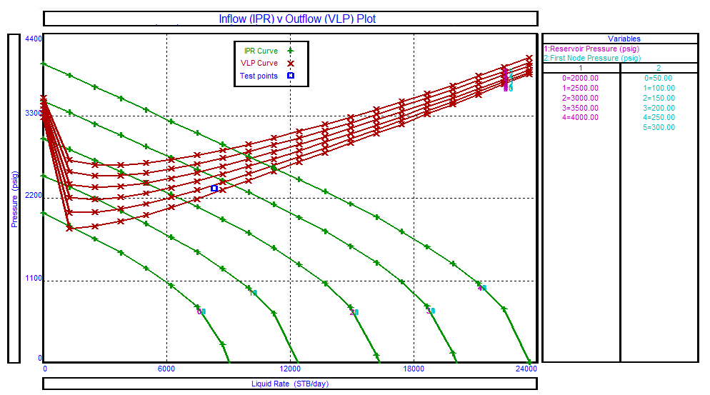
The intersection of WFP – Well Flow Performance and OPR curves represent the stabilized flow IPR and Lift Curves represent the Stabilised wellbore flow (see Fig. 1)
|
|
| Fig. 1. The stablised flow rate is represnted as A sample case of stabilised wellbore flow represented by junction point of WFP – Well Flow Performance and OPR curves IPR and Lift Curves. | Fig. 2. The dead well scenario. |
Given a tubing head pressure
| LaTeX Math Inline | ||
|---|---|---|
|
|
|
| Fig. |
| 3. A sample case |
| of stabilised wellbore flow |
| as function of formation pressure. | Fig. |
4.A sample case |
as function |
|
| Fig. 45. A bunch of IPRs IPRs at different formation pressures and TPRs at different THPs Lift Curves at different THPs. |
Workflow
...
- Check the current production rate against the production target from FDP
- If the diffference is big enough to justify the cost of production optimization (see point 8 below) then proceed to the step 3 below
- Assess formation pressure based on well tests
- Simulate IPR /OPR based LC based on the current WOR/GOR
- Calculate the stabilized flow bottom-hole pressure
- Gather the current bottom-hole pressure
LaTeX Math Inline body p_{wf} - Check up the calculation aganst the actual
LaTeX Math Inline body p_{wf} - Recommend the production optimisation activities to adjust bottom-hole pressure
:LaTeX Math Inline body p_{wf} - adjusting the choke at surface
- adjusting the pump settings from surface
- changing the pump depth
- changing the tubing size
- changing the pump
- adjusting the choke at surface
The above workflow is very simplistic and assumes single-layer formation with no cross-flow complications.
In practise, the WFP – Well Flow Performance analysis is often very tentative and production technologists spend some time experimenting with well regimes on well-by-well basis.
...
IPR – Inflow Performance Relation
IPR – Inflow Performance Relation represents the relation between the bottom-hole pressure
| LaTeX Math Inline | ||
|---|---|---|
|
| LaTeX Math Inline | ||
|---|---|---|
|
| LaTeX Math Block | ||||
|---|---|---|---|---|
| ||||
p_{wf} = p_{wf}(q) |
which may be non-linear.
...
The WFP – Well Flow Performance analysis is closely related to well PI – Productivity Index
| LaTeX Math Inline | ||
|---|---|---|
|
| LaTeX Math Block | ||||
|---|---|---|---|---|
| ||||
J_{sO} = \frac{q_O}{p_R-p_{wf}} |
for oil producer with oil flowrate
| LaTeX Math Inline | ||
|---|---|---|
|
| LaTeX Math Block | ||||
|---|---|---|---|---|
| ||||
J_s(q_G) = \frac{q_G}{p_R-p_{wf}} |
for gas producer with gas flowrate
| LaTeX Math Inline | ||
|---|---|---|
|
| LaTeX Math Block | ||||
|---|---|---|---|---|
| ||||
J_s(q_g) = \frac{q_{GI}}{p_{wf}-p_R} |
for gas injector with injection rate
at surface conditionsLaTeX Math Inline body q_{GI}
| LaTeX Math Block | ||||
|---|---|---|---|---|
| ||||
J_s(q_w) = \frac{q_{WI}}{p_R-p_{wf}} |
for water injector with injection rate
| LaTeX Math Inline | ||
|---|---|---|
|
where
...
| LaTeX Math Inline | ||
|---|---|---|
|
...
field-average formation pressure within the drainage area
| LaTeX Math Inline | ||
|---|---|---|
|
| LaTeX Math Inline | ||
|---|---|---|
|
Based on above defintions the aribitrary WFP – Well Flow Performance can be wirtten in a general form:
| LaTeX Math Block | ||||
|---|---|---|---|---|
| ||||
p_{wf} = p_R - \frac{q}{J_s} |
providing that
| LaTeX Math Inline | ||
|---|---|---|
|
...
| LaTeX Math Inline | ||
|---|---|---|
|
...
| LaTeX Math Inline | ||
|---|---|---|
|
...
| LaTeX Math Inline | ||
|---|---|---|
|
...
| LaTeX Math Inline | ||
|---|---|---|
|
...
| LaTeX Math Inline | ||
|---|---|---|
|
...
The Productivity Index can be constant or dependent on bottom-hole pressure
| LaTeX Math Inline | ||
|---|---|---|
|
| LaTeX Math Inline | ||
|---|---|---|
|
In general case of multiphase flow the PI
| LaTeX Math Inline | ||
|---|---|---|
|
| LaTeX Math Inline | ||
|---|---|---|
|
| LaTeX Math Inline | ||
|---|---|---|
|
For undersaturated reservoir the numerically-simulated WFP – Well Flow Performances have been approximated by analytical models and some of them are brought below.
These correlations are usually expressed in terms of
| LaTeX Math Inline | ||
|---|---|---|
|
| LaTeX Math Block Reference | ||
|---|---|---|
|
They are very helpful in practise to design a proper well flow optimization procedure.
These correaltions should be calibrated to the available well test data to set a up a customized WFP – Well Flow Performance model for a given formation.
Water and Dead Oil IPR
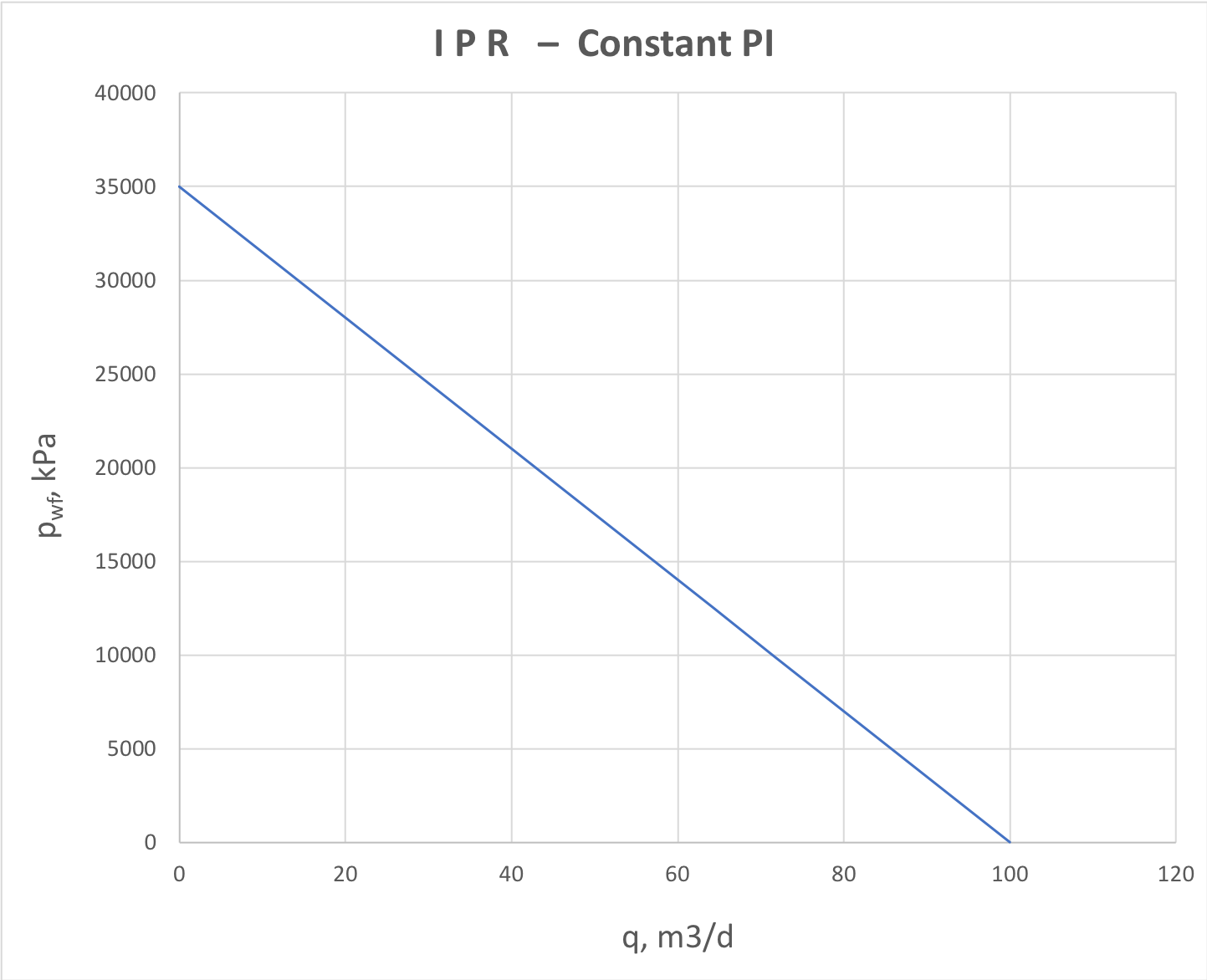
For a single layer formation with low-compressibility fluid (water or dead oil) the PI does not depend on drawdown (or flowrate)
| LaTeX Math Inline | ||
|---|---|---|
|
...
...
This is a typical WFP – Well Flow Performance plot for water supply wells, water injectors and dead oil producers.
The PI can be estimated using the Darcy equation:
| LaTeX Math Block | ||||
|---|---|---|---|---|
| ||||
J_s = \frac{2 \pi \sigma}{ \ln \frac{r_e}{r_w} + \epsilon+ S} |
where
| LaTeX Math Inline | ||
|---|---|---|
|
| LaTeX Math Block Reference | ||||
|---|---|---|---|---|
|
| LaTeX Math Inline | ||
|---|---|---|
|
| LaTeX Math Inline | ||
|---|---|---|
|
...
The alternative form of the constant Productivity Index WFP – Well Flow Performance is given by:
| LaTeX Math Block | ||||
|---|---|---|---|---|
| ||||
\frac{q}{q_{max}} = 1 -\frac{p_{wf}}{p_R} |
where
| LaTeX Math Inline | ||
|---|---|---|
|
Dry Gas IPR
For gas producers, the fluid compressibility is high and formation flow is essentially non-linear, inflicting the downward trend on the whole WFP – Well Flow Performance plot (Fig. 2).
...

...
Fig. 2. WFP – Well Flow Performance for dry gas producer or gas injector into a gas formation
The popular dry gas WFP – Well Flow Performance correlation is Rawlins and Shellhardt:
| LaTeX Math Block | ||||
|---|---|---|---|---|
| ||||
\frac{q}{q_{max}} = \Bigg[ \, 1- \Bigg( \frac{p_{wf}}{p_R} \Bigg)^2 \, \Bigg]^n |
where
| LaTeX Math Inline | ||
|---|---|---|
|
The more accurate approximation is given by LIT (Laminar Inertial Turbulent) IPR model:
| LaTeX Math Block | ||||
|---|---|---|---|---|
| ||||
a \, q + b \, q^2 = \Psi(p_R) - \Psi(p_{wf}) |
where
| LaTeX Math Inline | ||
|---|---|---|
|
| LaTeX Math Inline | ||
|---|---|---|
|
| LaTeX Math Inline | ||
|---|---|---|
|
It needs two well tests at two different rates to assess
| LaTeX Math Inline | ||
|---|---|---|
|
| LaTeX Math Inline | ||
|---|---|---|
|
But obviously more tests will make assessment more accruate.
Saturated Oil IPR
For saturated oil reservoir the free gas flow inflict the downward trend of WFP – Well Flow Performance plot similar to dry gas (Fig. 3).
...

...
Fig. 3. WFP – Well Flow Performance for 2-phase oil+gas production below and above bubble point
The analytical correlation for saturted oil flow is given by Vogel model:
| LaTeX Math Block | ||||
|---|---|---|---|---|
| ||||
\frac{q}{q_{max}} = 1 - 0.2 \, \frac{p_{wf}}{p_R} - 0.8 \Bigg(\frac{p_{wf}}{p_R} \Bigg)^2 \quad , \quad p_b > p_R > p_{wf} |
Undersaturated Oil IPR
For undersaturated oil reservoir
| LaTeX Math Inline | ||
|---|---|---|
|
When it is higher than bubble point
| LaTeX Math Inline | ||
|---|---|---|
|
When bottom-hole pressure goes below bubble point
| LaTeX Math Inline | ||
|---|---|---|
|
It can be interpreted as deterioration of near-reservoir zone permeability when the fluid velocity is high and approximated by rate-dependant skin-factor.
...

...
Fig. 3. WFP – Well Flow Performance for 2-phase oil+gas production below and above bubble point
The analytical correlation for undersaturated oil flow is given by modified Vogel model:
| LaTeX Math Block | ||||
|---|---|---|---|---|
| ||||
\frac{q}{q_b} = \frac{p_R - p_{wf}}{p_R - p_b} \quad , \quad p_R > p_{wf} > p_b |
| LaTeX Math Block | ||||
|---|---|---|---|---|
| ||||
q = (q_{max} - q_b ) \Bigg[ 1 - 0.2 \, \frac{p_{wf}}{p_b} - 0.8 \Bigg(\frac{p_{wf}}{p_b} \Bigg)^2 \Bigg] + q_b \quad , \quad p_R > p_b > p_{wf} |
with AOF
| LaTeX Math Inline | ||
|---|---|---|
|
| LaTeX Math Inline | ||
|---|---|---|
|
| LaTeX Math Block | ||||
|---|---|---|---|---|
| ||||
q_{max} = q_b \, \Big[1 + \frac{1}{1.8} \frac{p_b}{(p_r - p_b)} \Big] |
Saturated Multiphase IPR
For saturated 3-phase water-oil-gas reservoir the WFP – Well Flow Performance analysis is represented by oil and water components separately (see Fig. 4.1 and Fig. 4.2).
...

...

...
Fig. 4.1. Oil WFP – Well Flow Performance for saturated 3-phase (water + oil + gas) formation flow
...
Fig. 4.2. Water WFP – Well Flow Performance for saturated 3-phase (water + oil + gas) formation flow
The analytical correlation for saturated 3-phase oil flow is given by Wiggins model:
| LaTeX Math Block | ||||
|---|---|---|---|---|
| ||||
\frac{q_o}{q_{o, \, max}} = 1 - 0.52 \, \frac{p_{wf}}{p_R} - 0.48 \Bigg(\frac{p_{wf}}{p_R} \Bigg)^2 |
| LaTeX Math Block | ||||
|---|---|---|---|---|
| ||||
\frac{q_w}{q_{w, \, max}} = 1 - 0.72 \, \frac{p_{wf}}{p_R} - 0.28 \Bigg(\frac{p_{wf}}{p_R} \Bigg)^2 |
Undersaturated Multiphase IPR
For undersaturated 3-phase water-oil-gas reservoir the WFP – Well Flow Performance analysis is represented by oil and water components separately (see Fig. 4.1 and Fig. 4.2).
...

...

...
Fig. 4.1. Oil WFP – Well Flow Performance for udersaturated 3-phase (water + oil + gas) formation flow
...
Fig. 4.2. Water WFP – Well Flow Performance for undersaturated 3-phase (water + oil + gas) formation flow
...
| special | @self |
|---|
The analytical correlation for saturated 3-phase oil flow is given by Wiggins model:
| LaTeX Math Block | ||||
|---|---|---|---|---|
| ||||
\frac{q_o}{q_{o, \, max}} = 1 - 0.52 \, \frac{p_{wf}}{p_R} - 0.48 \Bigg(\frac{p_{wf}}{p_R} \Bigg)^2 |
| LaTeX Math Block | ||||
|---|---|---|---|---|
| ||||
\frac{q_w}{q_{w, \, max}} = 1 - 0.72 \, \frac{p_{wf}}{p_R} - 0.28 \Bigg(\frac{p_{wf}}{p_R} \Bigg)^2 |
See Also
...
Petroleum Industry / Upstream / Production / Subsurface Production / Well & Reservoir Management
Subsurface E&P Disciplines / Production Technology
[ Inflow Performance Relation (IPR) ] [ Lift Curves (LC) ]
...
OPR – Outflow Performance Relation
OPR – Outflow Performance Relation also called TPR – Tubing Performance Relation and VLP – Vertical Lift Performance represents the relation between the bottom-hole pressure
| LaTeX Math Inline | ||
|---|---|---|
|
| LaTeX Math Inline | ||
|---|---|---|
|
| LaTeX Math Block | ||||
|---|---|---|---|---|
| ||||
p_{wf} = p_{wf}(q) |
which may be non-linear.
...

...
...
| Anchor | ||||
|---|---|---|---|---|
|
References
...
Joe Dunn Clegg, Petroleum Engineering Handbook, Vol. IV – Production Operations Engineering, SPE, 2007
...