...
| Excerpt Include |
|---|
| Aquifer Drive |
|---|
| Aquifer Drive |
|---|
| nopanel | true |
|---|
|
Inputs & Outputs
...
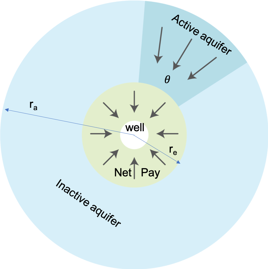
Physical Model
...
Mathematical Model
...
| Radial Drive | Linear drive |
|---|
| LaTeX Math Block |
|---|
| Q^{\downarrow}_{AQ}= B \cdot \int_0^t W_{eD} \left( \frac{(t-\tau)\chi}{r_e^2 |
|
}, \frac{r_a{r_e} \right) \dot p(\tau) d\tau |
| |
,r)= \int_0^{t} \frac{\partial p_1}{\partial r_D} \bigg|_{r |
|
_D = 1} dt_D | LaTeX Math Block |
|---|
|
Q^{\downarrow}_{AQ}= B \cdot \int_0^t W_{eD} \left( \frac{(t-\tau)\chi}{r_e^2}, \frac{r_a}{x_e} \right) \dot p(\tau) d\tau |
| LaTeX Math Block |
|---|
|
W_{eD}(t, r)= \int_0^{t} \frac{\partial p_1}{\partial x_D} \bigg|{x_anchor | | | LaTeX Math Block |
|---|
| q^{\downarrow}_{AQ}(t)= \frac{dQ^{\downarrow}_{AQ}}{dt} |
| | LaTeX Math Block |
|---|
| p_1 = p_1(t_D, r_D) |
|
|
1 | | alignment | left |
|---|
q^{\downarrow}_{AQ}(t)= \frac{dQ^{\downarrow}_{AQ}}{dt} |
| LaTeX Math Block |
|---|
|
p_1 = p_1(t_D, x_D) |
| LaTeX Math Block |
|---|
| \frac{\partial p_1}{\partial t_D} = \frac{\partial^2 p_1}{\partial r_D^2} + \frac{1}{r_D}\cdot \frac{\partial p_1}{\partial r_D} |
| | LaTeX Math Block |
|---|
| p_1(t_D = 0, r |
|
_D)= 0| LaTeX Math Block |
|---|
|
\frac{\partial p_1}{\partial t_D} = \frac{\partial^2 p_1}{\partial x_D^2} |
| LaTeX Math Block |
|---|
|
p_1(t_D = 0, x
| | LaTeX Math Block |
|---|
| p_1(t_D, r_D=1) = 1 |
| | LaTeX Math Block |
|---|
| \frac{\partial p_1(t_D, r_D)}{\partial r_D}
\Bigg|_{r_D=r_{aD}} = 0 |
or | LaTeX Math Block |
|---|
| p_1(t_D, r_D = \infty) = 0 |
|
| LaTeX Math Block |
|---|
| anchor | CT |
|---|
alignment | leftp_1(t_D, x_D=1) = 1 |
| LaTeX Math Block |
|---|
|
\frac{\partial p_1(t_D, x_D)}{\partial r_D}
\Bigg|_{x_D=x_{aD}} = 0 |
or
| LaTeX Math Block |
|---|
|
p_1(t_D, x_D = \infty) = 0 |
| Expand |
|---|
|
| Panel |
|---|
|
| borderColor | wheat |
|---|
| borderWidth | 10 |
|---|
|
Transient flow in Radial Composite Reservoir:
| LaTeX Math Block |
|---|
|
\frac{\partial p_a}{\partial t} = \chi \cdot \left[ \frac{\partial^2 p_a}{\partial r^2} + \frac{1}{r}\cdot \frac{\partial p_a}{\partial r} \right] |
| LaTeX Math Block |
|---|
|
p_a(t = 0, r)= p(0) |
| LaTeX Math Block |
|---|
|
p_a(t, r=r_e) = p(t) |
| LaTeX Math Block |
|---|
| anchor | p1_PSS |
|---|
| alignment | left |
|---|
|
\frac{\partial p_a}{\partial r}
\bigg|_{(t, r=r_a)} = 0 |
Consider a pressure convolution:
| LaTeX Math Block |
|---|
|
p_a(t, r) = p(0) + \int_0^t p_1 \left(\frac{(t-\tau) \cdot \chi}{r_e^2}, \frac{r}{r_e} \right) \dot p(\tau) d\tau |
| LaTeX Math Block |
|---|
|
\dot p(\tau) = \frac{d p}{d \tau} |
One can easily check that
| LaTeX Math Block Reference |
|---|
|
honors the whole set of equations | LaTeX Math Block Reference |
|---|
|
–| LaTeX Math Block Reference |
|---|
|
and as such defines a unique solution of the above problem.Water flowrate within
sector angle at interface with oil reservoir will be:| LaTeX Math Block |
|---|
|
q^{\downarrow}_{AQ}(t)= \theta \cdot r_e \cdot h \cdot u(t,r_e) |
where
is flow velocity at aquifer contact boundary, which is:| LaTeX Math Block |
|---|
|
u(t,r_e) = M \cdot \frac{\partial p_a(t,r)}{\partial r} \bigg|_{r=r_e} |
where
is aquifer mobility.Water flowrate becomes:
| LaTeX Math Block |
|---|
|
q^{\downarrow}_{AQ}(t)= \theta \cdot r_e \cdot h \cdot M \cdot \frac{\partial p_a(t,r)}{\partial r} \bigg|_{r=r_e} |
Cumulative water flux:
| LaTeX Math Block |
|---|
|
Q^{\downarrow}_{AQ}(t) = \int_0^t q^{\downarrow}_{AQ}(t) dt = \theta \cdot r_e \cdot h \cdot M \cdot \int_0^t \frac{\partial p_a(t,r)}{\partial r} \bigg|_{r=r_e} dt |
Substituting
| LaTeX Math Block Reference |
|---|
|
into | LaTeX Math Block Reference |
|---|
|
leads to:| LaTeX Math Block |
|---|
|
Q^{\downarrow}_{AQ}(t) = \theta  \cdot r_e \cdot h \cdot M  \cdot \int_0^t d\xi \  \frac{\partial }{\partial r} \left[

\int_0^\xi p_1 \left( \frac{(\xi-\tau)\chi}{r_e^2}, \frac{r}{r_e} \right) \, \dot p(\tau) d\tau

\right]_{r=r_e} |
| LaTeX Math Block |
|---|
|
Q^{\downarrow}_{AQ}(t) = \theta  \cdot h \cdot M  \cdot \int_0^t d\xi \  \frac{\partial }{\partial r_D} \left[

\int_0^\xi p_1 \left( \frac{(\xi-\tau)\chi}{r_e^2}, r_D \right) \, \dot p(\tau) d\tau

\right]_{r_D=1} |
| LaTeX Math Block |
|---|
|
Q^{\downarrow}_{AQ}(t) = \theta  \cdot h \cdot M  \cdot \int_0^t d\xi \

\int_0^\xi \frac{\partial p_1}{\partial r_D} \left( \frac{(\xi-\tau)\chi}{r_e^2}, r_D \right) \Bigg|_{r_D=1} \, \dot p(\tau) d\tau
|
The above integral represents the integration over the
area in plane (see Fig. 1):| LaTeX Math Block |
|---|
|
Q^{\downarrow}_{AQ}(t) = \theta  \cdot h \cdot M  \cdot \iint_D d\xi \ d\tau  \, \dot p(\tau)

\frac{\partial p_1}{\partial r_D} \left( \frac{(\xi-\tau)\chi}{r_e^2}, r_D \right) \Bigg|_{r_D=1}
|
 Image Removed Image Removed
|
Fig. 1. Illustration of the integration area in plane |
Changing the integration order from
to leads to:| LaTeX Math Block |
|---|
|
Q^{\downarrow}_{AQ}(t) = \theta  \cdot h \cdot M  \cdot \int_0^t d\tau \int_\tau^t d\xi  \ \dot p(\tau)

\frac{\partial p_1}{\partial r_D} \left( \frac{(\xi-\tau)\chi}{r_e^2}, r_D \right) \Bigg|_{r_D=1}
=
 \theta  \cdot h \cdot M  \cdot \int_0^t \dot p(\tau) d\tau \int_\tau^t d\xi  \

\frac{\partial p_1}{\partial r_D} \left( \frac{(\xi-\tau)\chi}{r_e^2}, r_D \right) \Bigg|_{r_D=1} |
Replacing the variable:
| LaTeX Math Block |
|---|
|
\xi = \tau + \frac{r_e^2}{\chi} \cdot t_D \rightarrow t_D = \frac{(\xi-\tau)\chi}{r_e^2} \rightarrow d\xi = \frac{r_e^2}{\chi} \cdot dt_D |
and flux becomes:
| LaTeX Math Block |
|---|
|
Q^{\downarrow}_{AQ}(t) = \theta  \cdot h \cdot M \cdot \frac{r_e^2}{\chi} \cdot \int_0^t \dot p(\tau) d\tau \int_0^{(t-\tau)\chi/r_e^2}

\frac{\partial p_1( t_D, r_D)}{\partial r_D}  \Bigg|_{r_D=1} dt_D = B \cdot \int_0^t \dot p(\tau) d\tau \int_0^{(t-\tau)\chi/r_e^2}

\frac{\partial p_1( t_D, r_D)}{\partial r_D} \Bigg|_{r_D=1} dt_D |
where is water influx constant and which leads to | LaTeX Math Block Reference |
|---|
|
and | LaTeX Math Block Reference |
|---|
|
.Derivation of Radial VEH Aquifer Drive @model
Computational Model
...
| LaTeX Math Block |
|---|
| Q^{\downarrow}_{AQ}(t)= B \cdot \sum_\alpha W_{eD}
\left( \frac{ (t-\tau_\alpha) \chi}{r_e^2} |
|
,frac{r_a}{r_e} \right)\Delta p_\alpha
= B \cdot W_{eD}
\left( \frac{ (t-\tau_1) \chi}{r_e^2 |
|
}, \frac{r_a{r_e} \right)\Delta p_1 +
B \cdot W_{eD}
\left( \frac{ (t-\tau_2) \chi}{r_e^2 |
|
}, \frac{r_a}{r_e} \right)\Delta p_2
+ ... + B \cdot W_{eD}
\left( \frac{ (t-\tau_N) \chi}{r_e^2} |
|
, \frac{r_a}{r_e} This computational model is using a discrete convolution (also called superposition in some publications) with time-grid
| LaTeX Math Inline |
|---|
| body | \{ \tau_1, \, \tau_2, \ ... \ , \tau_N \} |
|---|
|
.
...
| Expand |
|---|
| title | Polynomial approximations for WeD |
|---|
|
Polynomial approximation of are available (http://dx.doi.org/10.2118/15433-PA).
Table 1. Polynomial approximation of for infinite aquifer | | LaTeX Math Inline |
|---|
| body | W_{eD}=\sqrt{\frac{t_D}{\pi}} |
|---|
|
| | | LaTeX Math Inline |
|---|
| body | \displaystyle W_{eD}=\frac {1.2838 \cdot t_D^{1/2} + 1.19328 \cdot t_D +0.269872 \cdot t_D^{3/2} +0.00855294 \cdot t_D^2} {1+0.616599 \cdot t_D^{1/2}+0.0413008 \cdot t_D} |
|---|
|
| | | LaTeX Math Inline |
|---|
| body | \displaystyle W_{eD}=\frac{-4.29881+2.02566 \cdot t_D}{\ln t_D} |
|---|
|
|
|
Scope of Applicability
...
The benefit of VEH approach is that net pay formation pressure history
is usually known so that water influx calculation based on aquifer properties
| LaTeX Math Inline |
|---|
| body | \{ B, \, r_a, \, \chi \} |
|---|
|
is rather straightforward.
...
In modern computers the convolution is a fast fully-automated procedure and VEH model is considered as a reference in the range of analytical aquifer models.
Although the model is derived for linear and radial flow it also shows a good match for bottom-water drive depletions.
...