Motivation
...
| Excerpt Include |
|---|
| Aquifer Drive |
|---|
| Aquifer Drive |
|---|
| nopanel | true |
|---|
|
Inputs & Outputs
...
...
...
...
...
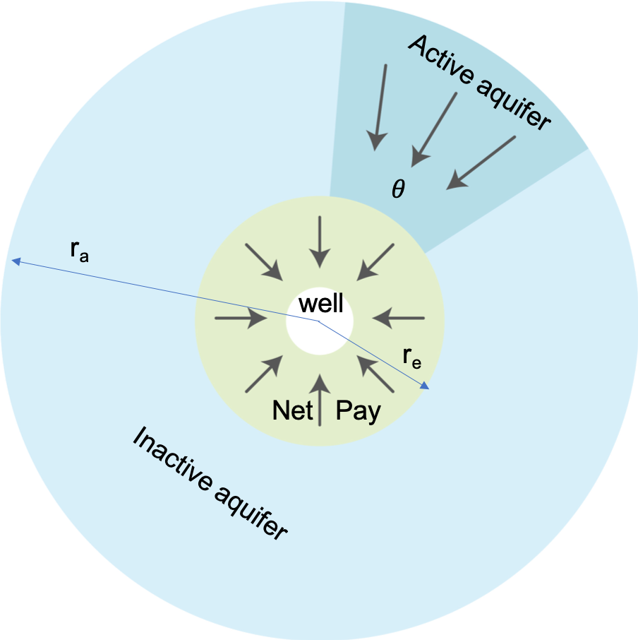
Physical Model
...
 Image Removed Image Removed
|
Mathematical Model
...
| LaTeX Math Block |
|---|
| Q^{\downarrow}_{AQ}= B \cdot \int_0^t W_{eD} \left( \frac{(t-\tau)\chi |
|
_a, frac{r_a}{r_e} \right) \dot p(\tau) d\tau |
| |
1| alignment | left |
|---|
q^{\downarrow}_{AQ}(t)= \frac{dQ^{\downarrow}_{AQ}}{dt} |
| LaTeX Math Block |
|---|
anchor | ,r)= \int_0^{t} \frac{\partial p_1}{\partial r_D} \bigg|_{r_D = 1} dt_D |
| |
RC1\fracpartial p_1}{\partial t_D} = downarrow}_{AQ}(t)= \frac{ |
|
\partial^2 p_1}{\partial r_D^2} + \frac{1}{r_D}\cdot \frac{\partial p_1}{\partial r_DdQ^{\downarrow}_{AQ}}{dt} |
| |
CT(t_D =0, r_D)0| LaTeX Math Block |
|---|
|
=1 = 11 | \frac{\partial p_1}{\partial |
|
r_D}
\bigg|_{(, r_D=r_a/r_e)0...
...
Transient flow in Radial Composite Reservoir:
...
...
...
...
...
...
r_D^2} + \frac{1}{r_D}\cdot \frac{\partial p_ |
|
...
...
...
...
...
...
...
...
...
...
...
...
_1(t_D, r_D)}{\partial r_D}
\ |
|
...
...
...
...
...
...
...
...
...
...
...
...
| LaTeX Math Block |
|---|
|
\dot p(\tau) = \frac{d p}{d \tau} |
One can easily check that
| LaTeX Math Block Reference |
|---|
|
honors the whole set of equations | LaTeX Math Block Reference |
|---|
|
–| LaTeX Math Block Reference |
|---|
|
and as such defines a unique solution of the above problem.Water flowrate within
sector angle at interface with oil reservoir will be:...
...
Computational Model
...
| LaTeX Math Block |
|---|
| Q^{\downarrow}_{AQ}(t)= |
|
...
...
where
is flow velocity at aquifer contact boundary, which is:| LaTeX Math Block |
|---|
|
u(t,r_e) = M_a \cdot \frac{\partial p_a(t,r)}{\partial r} \bigg|_{r=r_e} |
where
| LaTeX Math Inline |
|---|
| body | M_a = \frac{k_a}{\mu_w} |
|---|
|
is aquifer mobility.Water flowrate becomes:
| LaTeX Math Block |
|---|
|
q^{\downarrow}_{AQ}(t)= \theta \cdot r_e \cdot h_a \cdot M_a \cdot \frac{\partial p_a(t,r)}{\partial r} \bigg|_{r=r_e} |
Cumulative water flux:
| LaTeX Math Block |
|---|
|
Q^{\downarrow}_{AQ}(t) = \int_0^t q^{\downarrow}_{AQ}(t) dt = \theta \cdot r_e \cdot h_a \cdot M_a \cdot \int_0^t \frac{\partial p_a(t,r)}{\partial r} \bigg|_{r=r_e} dt |
Substituting
| LaTeX Math Block Reference |
|---|
|
into | LaTeX Math Block Reference |
|---|
|
leads to:...
...
\sum_\alpha W_{eD}
\left( \frac{ (t-\tau_\alpha) \chi}{r_e^2} \right)\Delta p_\alpha


= B \cdot W_{eD}
\left( \frac{ ( |
|
...
...
...
...
...
...
...
...
...
...
...
...
...
...
...
...
...
...
...
p_2
+ ... + B \cdot W_{eD}
\left( \frac{ ( |
|
...
...
...
...
...
The above integral represents the integration over the
area in plane (see Fig. 1):| LaTeX Math Block |
|---|
|
Q^{\downarrow}_{AQ}(t) = \theta  \cdot h_a \cdot M_a  \cdot \iint_D d\xi \ d\tau  \, \dot p(\tau)

\frac{\partial p_1}{\partial r_D} \left( \frac{(\xi-\tau)\chi_a}{r_e^2}, r_D \right) \Bigg|_{r_D=1}
|
...
 Image Removed
...
Fig. 1. Illustration of the integration
area in planeChanging the integration order from
to leads to:| LaTeX Math Block |
|---|
|
Q^{\downarrow}_{AQ}(t) = \theta  \cdot h_a \cdot M_a  \cdot \int_0^t d\tau \int_\tau^t d\xi  \ \dot p(\tau)

\frac{\partial p_1}{\partial r_D} \left( \frac{(\xi-\tau)\chi_a}{r_e^2}, r_D \right) \Bigg|_{r_D=1}
=
 \theta  \cdot h_a \cdot M_a  \cdot \int_0^t \dot p(\tau) d\tau \int_\tau^t d\xi  \

\frac{\partial p_1}{\partial r_D} \left( \frac{(\xi-\tau)\chi_a}{r_e^2}, r_D \right) \Bigg|_{r_D=1} |
Replacing the variable:
| LaTeX Math Block |
|---|
|
\xi = \tau + \frac{r_e^2}{\chi_a} \cdot t_D \rightarrow t_D = \frac{(\xi-\tau)\chi_a}{r_e^2} \rightarrow d\xi = \frac{r_e^2}{\chi_a} \cdot dt_D |
and flux becomes:
| LaTeX Math Block |
|---|
|
Q^{\downarrow}_{AQ}(t) = \theta  \cdot h_a \cdot M_a \cdot \frac{r_e^2}{\chi_a} \cdot \int_0^t \dot p(\tau) d\tau \int_0^{(t-\tau)\chi_a/r_e^2}

\frac{\partial p_1( t_D, r_D)}{\partial r_D} \Bigg|_{r_D=1} dt_D |
and finally:
| LaTeX Math Block |
|---|
|
Q^{\downarrow}_{AQ}(t) = \theta  \cdot h_a \cdot M_a \cdot \frac{r_e^2}{\chi_a} \cdot \int_0^t \dot p(\tau) d\tau \int_0^{(t-\tau)\chi_a/r_e^2}

\frac{\partial p_1( t_D, r_D)}{\partial r_D} \Bigg|_{r_D=1} dt_D |
which leads to
| LaTeX Math Block Reference |
|---|
|
and | LaTeX Math Block Reference |
|---|
|
.Computational Model
| LaTeX Math Block |
|---|
|
Q^{\downarrow}_{AQ}(t)= B \cdot \sum_\alpha W_{eD}
\left( \frac{ (t-\tau_\alpha) \chi_a}{r_e^2}, \frac{r_a}{r_e}  \right)\Delta p_\alpha


= B \cdot W_{eD}
\left( \frac{ (t-\tau_1) \chi_a}{r_e^2}, \frac{r_a}{r_e}  \right)\Delta p_1 +
 B \cdot W_{eD}
\left( \frac{ (t-\tau_2) \chi_a}{r_e^2}, \frac{r_a}{r_e}  \right)\Delta p_2
+ ... + B \cdot W_{eD}
\left( \frac{ (t-\tau_N) \chi_a}{r_e^2}, \frac{r_a}{r_e} \right)\Delta p_N |
This computational scheme is called superposition in time domain.
...
This computational model is using a discrete convolution (also called superposition in some publications) with time-grid
| LaTeX Math Inline |
|---|
| body | \{ \tau_1, \, \tau_2, \ ... \ , \tau_N \} |
|---|
|
.In practical exercises with manual or spreadsheet-assisted calculations the time-grid is usually uniform:
| LaTeX Math Inline |
|---|
| body | \{ \tau_1 =\Delta \tau, \, \tau_2 = 2 \cdot \Delta \tau, \ ... \ , \tau_N = N \cdot \Delta \tau\} |
|---|
|
with the time step of a month to ensure the formation pressure does not change much since the previous time step.Moving to annual time step may accumulate a substantial mistake if formation pressure has varied substantially in some years.
| Expand |
|---|
| title | Polynomial approximations for WeD |
|---|
|
Polynomial approximation of are available (http://dx.doi.org/10.2118/15433-PA).
Table 1. Polynomial approximation of for infinite aquifer | | LaTeX Math Inline |
|---|
| body | W_{eD}=\sqrt{\frac{t_D}{\pi}} |
|---|
|
| | | LaTeX Math Inline |
|---|
| body | \displaystyle W_{eD}=\frac {1.2838 \cdot t_D^{1/2} + 1.19328 \cdot t_D +0.269872 \cdot t_D^{3/2} +0.00855294 \cdot t_D^2} {1+0.616599 \cdot t_D^{1/2}+0.0413008 \cdot t_D} |
|---|
|
| | | LaTeX Math Inline |
|---|
| body | \displaystyle W_{eD}=\frac{-4.29881+2.02566 \cdot t_D}{\ln t_D} |
|---|
|
|
|
Scope of Applicability
...
The benefit of VEH approach is that net pay formation pressure history
is usually known
and the aquifer drive model parameters so that water influx calculation based on aquifer properties | LaTeX Math Inline |
|---|
| body | \{ B, \, r_a, \, \chi \} |
|---|
|
can be calibrated iteratively by using | LaTeX Math Block Reference |
|---|
|
in Material Balance calculations is rather straightforward.In the past the VEH approach was considered as tedious in calculating superposition during the manual exercises.
In modern computers the convolution is a fast fully-automated procedure and VEH model is considered as a reference in the range of analytical aquifer models.
Although the model is derived for linear and radial flow it also shows a good match for bottom-water drive depletions.
See Also
...
Petroleum Industry / Upstream / Subsurface E&P Disciplines / Field Study & Modelling / Aquifer Drive / Aquifer Drive Models
Reference
...
1. van Everdingen, A.F. and Hurst, W. 1949. The Application of the Laplace Transformation to Flow Problems in Reservoirs. Trans., AIME 186, 305.
...

