...
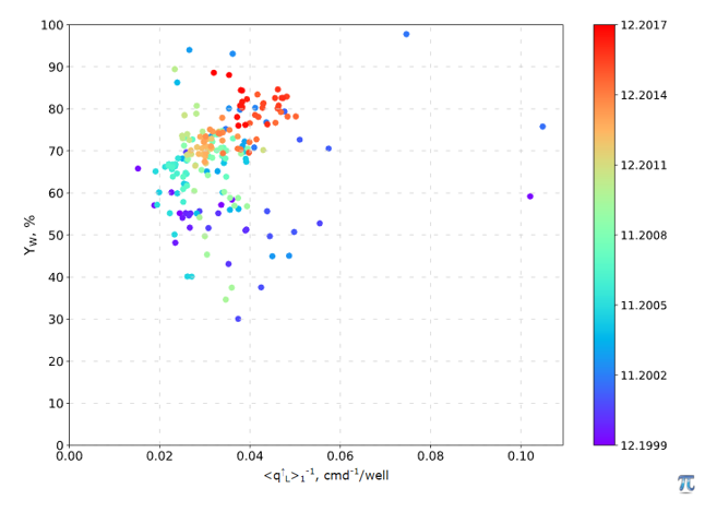
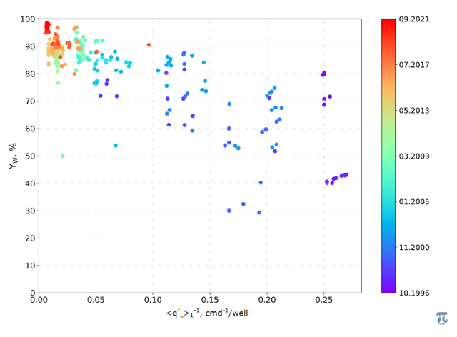
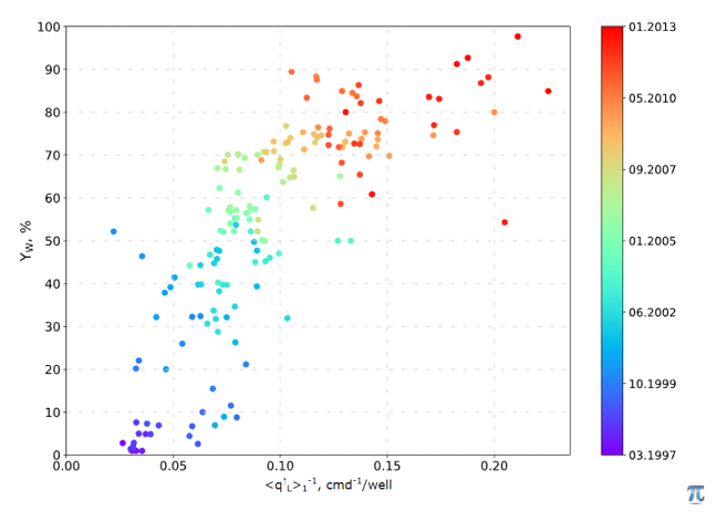
One if the Watercut Diagnostics plots with water cut (Yw) along y-axis and inverse liquid rate
along x-axis (see
Fig. 1 –
Fig. 3).
...
The mathematical model of the thief water production from aquifer is based on the following equation:
| LaTeX Math Block |
|---|
| Y_W = a + b |
|
/ q | | LaTeX Math Block |
|---|
| a = \frac{J_{1W} + J_{2W}}{J_{1O} + J_{1W} + J_{2W}} |
| | LaTeX Math Block |
|---|
| b = \frac{J_{1O} \cdot J_{2W}}{J_{1O} + J_{1W} + J_{2W}} \cdot (p^*_2 - p^*_1) |
|
where
The equation
| LaTeX Math Block Reference |
|---|
|
suggests that water cut declines along with aquifer pressure decline.It also suggest that water cut grows with decline of the petroleum reservoir pressure and decreases when petroleum reservoir pressure grows.
For the case of aquifer pressure is higher than that of petroleum reservoir:
| LaTeX Math Inline |
|---|
| body | --uriencoded--b > 0 \Leftrightarrow p%5e*_2 > p%5e*_1 |
|---|
|
,which means that if aquifer pressure is higher than petroleum reservoir pressure then production increase will lead to the water cut decline.
For the case of aquifer pressure is lower than that of petroleum reservoir:
| LaTeX Math Inline |
|---|
| body | --uriencoded--b < 0 \Leftrightarrow p%5e*_2 < p%5e*_1 |
|---|
|
,which means that if aquifer pressure is lower than petroleum reservoir pressure then production increase will lead to the water cut growth.
In practical applications, the equation
| LaTeX Math Block Reference |
|---|
|
is often considered through the
weighted average values:
| LaTeX Math Block |
|---|
|
<qY_W>W = a\frac{ \,langle q_W \cdot <q_O> +rangle}{\langle q_L \rangle} = a + b \, b\cdot \langle q_L \rangle^{-1} |
where
<q_W> <q_O> | are weighted average of and |
There are different ways to calculate weighted average of the dynamic variable, for example:
<>\rangle_t \ = \frac{1}{t} \int_o^t A(t) \, dt |
| |
<A>\langle A \rangle_q \ = \frac{1}{Q(t)} \int_o^t A(t) \, q(t) \, dt |
|
Cases
...
Case 1
...