Motivation
The Temperature Flat Source Solution @model is one of the fundamental solutions of temperature diffusion equations modelling the temperature conduction in linear direction (see Fig. 1).
...
Subsurface Temperature Profile around Lateral Flow makes adjustments to Geothermal Temperature Profile
to account for the lateral reservoir flow with a constant temperature (see Fig. 1 and Fig. 2).
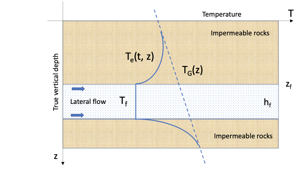 Image Added Image Added
| 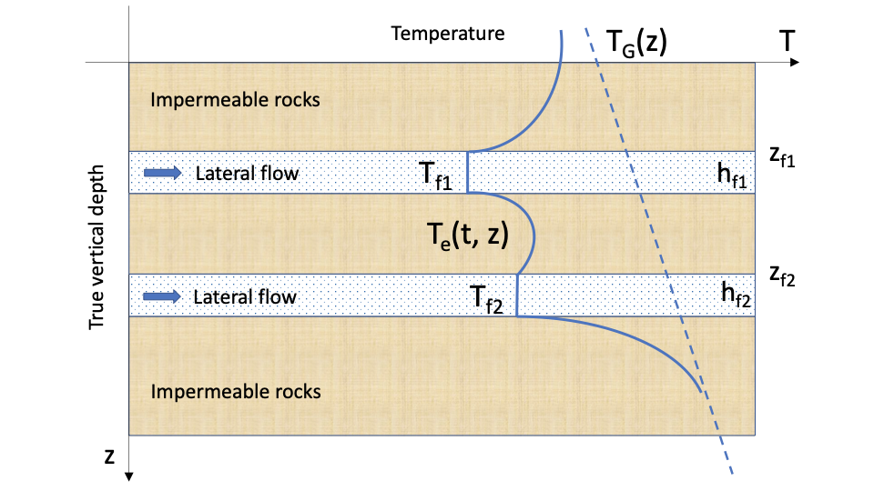 Image Added Image Added
|
Fig. 1. Sample Subsurface Temperature Profile around a height lateral flow at depth with temperature | Fig. 2. Sample Subsurface Temperature Profile around two lateral flows with temperature | LaTeX Math Inline |
|---|
| body | --uriencoded--T_%7Bf1%7D |
|---|
|
and | LaTeX Math Inline |
|---|
| body | --uriencoded--T_%7Bf2%7D |
|---|
|
|
Outputs
...
| Subsurface temperature distribution |
Inputs
...
| Time lapse after the temperature step from up to |
| Spatial coordinate along the transversal direction to constant temperature plane |
| TVDss of the top of the lateral flow unit |
| True vertical thickness of the the lateral flow unit |
| |
| Thermal diffusivity of the surroundings |
|
...
Equations
...
| Driving equation | Initial conditions | Boundary conditions |
|---|
| LaTeX Math Block |
|---|
| \frac{\partial T_e}{\partial t} = a_e^2 \, \Delta T_e = a_e^2 \, \frac{\partial^2 T_e}{\partial z^2} |
|
| LaTeX Math Block |
|---|
| T_e(t=0, z) = T_G(z) |
|
| LaTeX Math Block |
|---|
| T_e(t, z_f \leq z \leq z_f + h_f) = T_f = {\rm const} |
| LaTeX Math Block |
|---|
| T_e(t, z \rightarrow \infty) = |
|
...
Solution
...
Outputs
...
...
| \mbox{if} \, z < z_f \; \Longrightarrow \;T_e(t,z) = T_f + (T_G(z) - T_f) \cdot \mbox{erf} \left( \frac{z_f-z}{\sqrt{4 a_e t}} \right) |
|
| LaTeX Math Block |
|---|
| \mbox{if} \, z_f \leq z \leq z_f + h_f \; \Longrightarrow \; T_e(t,z) = T_f |
|
| LaTeX Math Block |
|---|
| \mbox{if} \, z > z_f + h_f \; \Longrightarrow \; T_e(t,z) = T_f + (T_G(z) - T_f) \cdot \mbox{erf} \left( \frac{z-z_f-h_f}{\sqrt{4 a_e t}} \right) |
|
where
See Also
...
Geology / Geothermal Temperature Field / Geothermal Temperature Profile
Physics / Fluid Dynamics / Linear Fluid Flow
[ Temperature Flat Source Solution @model ] [ Geothermal Temperature Profile @model ]
Reference
...
Inputs
...
| Heat flow equation for Semispace Linear Conduction: | LaTeX Math Block |
|---|
| \frac{\partial T}{\partial t} = a^2 \Delta T = a^2\frac{\partial^2 T}{\partial z^2} |
Initial Conditions | LaTeX Math Block |
|---|
| T(t=0, z) = T_G(z) |
Boundary conditions | LaTeX Math Block |
|---|
| T(t, z=0) = T_f = {\rm const}, \quad T(t, z \rightarrow \infty) = T_G(z) |
The exact solution is given by following formula: | LaTeX Math Block |
|---|
| T(t,z) = T_f + (T_G(z) - T_f) \cdot \frac{2}{\sqrt{\pi}} \int_0^{z/\sqrt{4at}} e^{-\xi^2} d\xi |
A fair approximation at late times ( ) is given by expanding the integral:| LaTeX Math Block |
|---|
| T(t,z) = T_f + (T_G(z) - T_f) \cdot \Bigg[ 1- \frac{\exp(-\zeta^2)}{\sqrt{\pi} \zeta} \bigg( 1- \frac{1}{2 \zeta} + \frac{3}{4 \zeta^3} \bigg) \Bigg] |
where | LaTeX Math Block |
|---|
| \zeta = \frac{z}{4 a t} |
The final solution for temperature above the flowing unit is represented by RHK pipe flow solution where TG is replaced with Tb from | LaTeX Math Block Reference |
|---|
|
.
For the intervals between two injection units the one needs to account for the SLC contribution from upper flowing unit and from lower flowing unit which can be done using the superposition.
First, let's rewrite | LaTeX Math Block Reference |
|---|
|
in terms of temperature gain:| LaTeX Math Block |
|---|
| dT(t, z) = T(t,z) - T_G(z)= - (T_G(z) - T_f) \cdot \frac{\exp(-\zeta^2)}{\sqrt{\pi} \zeta} \bigg( 1- \frac{1}{2 \zeta} + \frac{3}{4 \zeta^3} \bigg) |
Now one can write down the temperature disturbance from the overlying flowing unit A1: | LaTeX Math Block |
|---|
| dT_{b,over}(t, z) = T_{b,up}(t,z) - T_G(z)= - (T_G(z) - T_{f, A1}) \cdot \frac{\exp(-\zeta^2)}{\sqrt{\pi} \zeta} \bigg( 1- \frac{1}{2 \zeta} + \frac{3}{4 \zeta^3} \bigg) |
and from the underlying flowing unit A2: | LaTeX Math Block |
|---|
| dT_{b,under}(t, z) = T_{b,up}(t,z) - T_G(z)= - (T_G(z) - T_{f, A2}) \cdot \frac{\exp(-\zeta^2)}{\sqrt{\pi} \zeta} \bigg( 1- \frac{1}{2 \zeta} + \frac{3}{4 \zeta^3} \bigg) |
The background temperature disturbance between the flowing units will be: | LaTeX Math Block |
|---|
| T_b(t, z) = T_G(z) + dT_{b,over}(t, z) + dT_{b,under}(t, z) |
Replacing the static value of in RHK model with dynamic value of one arrives to the final wellbore temperature model with account of heat exchange with surrounding rocks and cooling effects from flowing units (Semispace Linear Conduction). |
|
|
...
See also
Physics / Fluid Dynamics / Linear Fluid Flow
References