The relation between the bottom-hole pressure
and surface flow rate
during the
stabilised formation flow:
| LaTeX Math Block |
|---|
|
p_{wf} = p_{wf}(q) |
which may be linear (Fig. 1) or non-linear (Fig. 2).
Widely used in Well Flow Performance analysis.
The IPR (Inflow Performance Relation) analysis is closely related to well Productivity Index (PI)
which is defined as below:
| LaTeX Math Block |
|---|
| J_{sO} = \frac{q_O}{p_r-p_{wf}} |
|
for oil producer with oil flowrate at surface conditions |
| LaTeX Math Block |
|---|
| J_s(q_G) = \frac{q_G}{p_r-p_{wf}} |
|
for gas producer with gas flowrate at surface conditions |
| LaTeX Math Block |
|---|
| J_s(q_g) = \frac{q_{GI}}{p_{wf}-p_r} |
|
for gas injector with injection rate at surface conditions |
| LaTeX Math Block |
|---|
| J_s(q_w) = \frac{q_{WI}}{p_r-p_{wf}} |
|
for water injector with injection rate at surface conditions |
where
| field-average formation pressure within the drainage area of a given well: | LaTeX Math Inline |
|---|
| body | p_r = \frac{1}{V_e} \, \int_{V_e} \, p(t, {\bf r}) \, dV |
|---|
|
|
Based on above defintions the aribitrary IPR can be wirtten in a general form:
| LaTeX Math Block |
|---|
|
p_{wf} = p_r - \frac{q}{J_s} |
providing that
has a specific meaning and sign as per the table below:
| for producer |
| for injector |
| for oil producer |
| for gas producer or injector |
| for water injector or water producer or water production from oil producer |
See more on the variations of PI definition between Dynamic Modelling, Well Flow Performance and Well Testing.
The Productivity Index can be constant (showing a straight line on IPR like on Fig. 1) or dependent on bottom-hole pressure
or equivalently on flowrate
(showing a curved line on
IPR like on
Fig. 2) .
In general case of multiphase flow the PI
features a complex dependance on bottom-hole pressure
(or equivalently on flowrate
) which can be etstablished based on numerical simulations of multiphase formation flow.
For undersaturated reservoir the numerically-simulated IPR (Inflow Performance Relation)s have been approximated by analytical models and some of them are brought below.
These correlations are usually expressed in terms of
as alternative to
| LaTeX Math Block Reference |
|---|
|
.
They are very helpful in practise to design a proper well flow optimization procedure.
These correaltions should be calibrated to the available well test data to set a up a customised IPR model for a given formation.
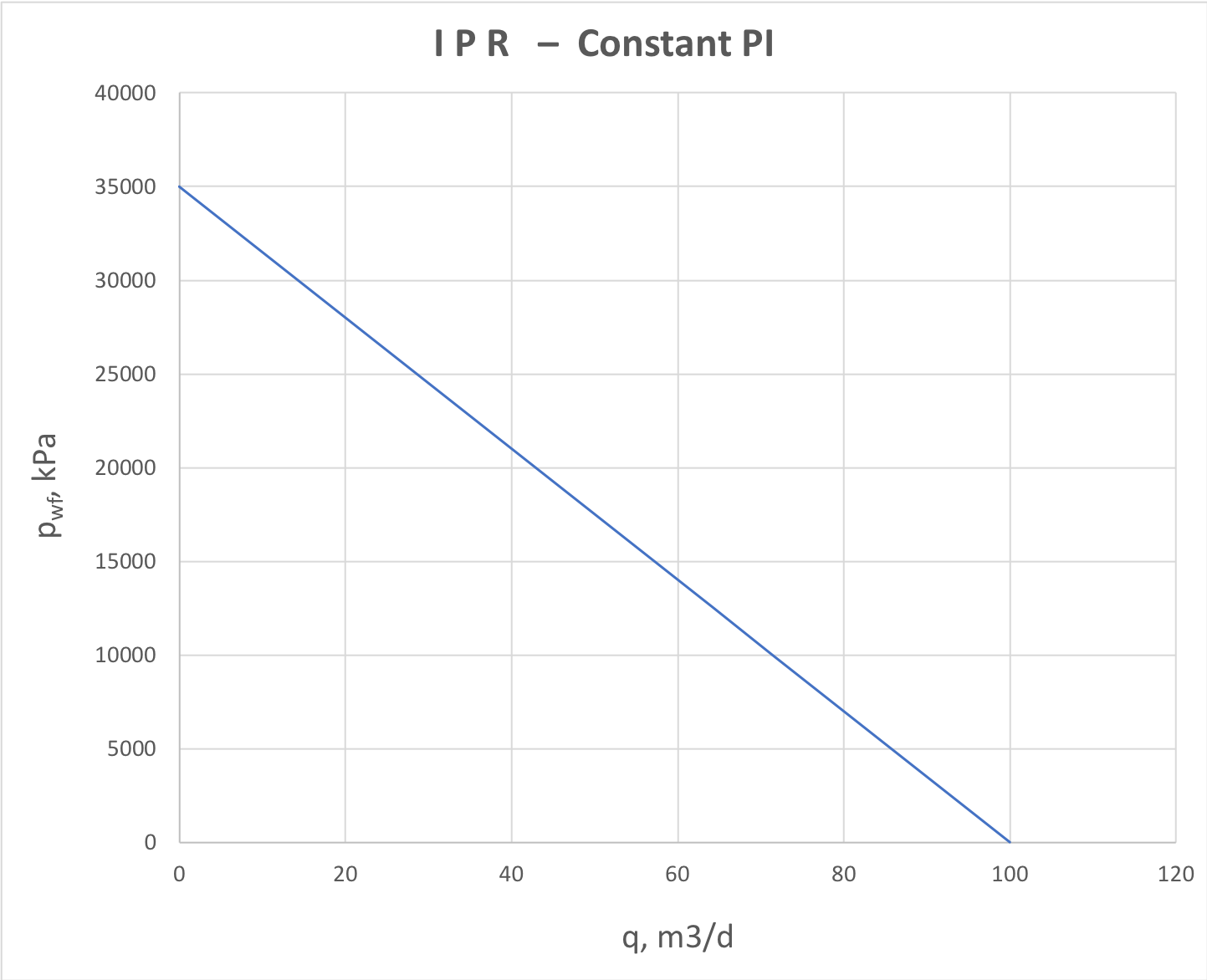
For a single layer formation with low-compressibility fluid (water or dead oil) the PI does not depend on drawdown (or flowrate)
and
IPR plot is reperented by a straight line (Fig. 1)
|
| Fig.1. IPR plot for constant productivity (water and dead oil) |
This is a typical IPR plot for water supply wells, water injectors and dead oil producers.
The PI can be estimated using the Darcy equation:
| LaTeX Math Block |
|---|
|
J_s = \frac{2 \pi \sigma}{ \ln \frac{r_e}{r_w} + \epsilon+ S} |
where
| LaTeX Math Inline |
|---|
| body | \sigma = \Big \langle \frac{k} {\mu} \Big \rangle \, h = k \, h\, \Big[ \frac{k_{rw}}{\mu_w} + \frac{k_{ro}}{\mu_o} \Big] |
|---|
|
– water-based or water-oil-based transmissbility above bubble point
| LaTeX Math Block Reference |
|---|
| anchor | Perrine2phase_alpha |
|---|
| page | Linear Perrine multi-phase diffusion (model) |
|---|
|
,
for steady-state
SS flow and
for pseudo-steady state
PSS flow.
The alternative form of the constant Productivity Index IPR is given by:
| LaTeX Math Block |
|---|
|
\frac{q}{q_{max}} = 1 -\frac{p_{wf}}{p_Rr} |
where
is the maximum reservoir deliverability when the bottom-hole is at atmospheric pressure and also called
Absolute Open Flow (AOF).
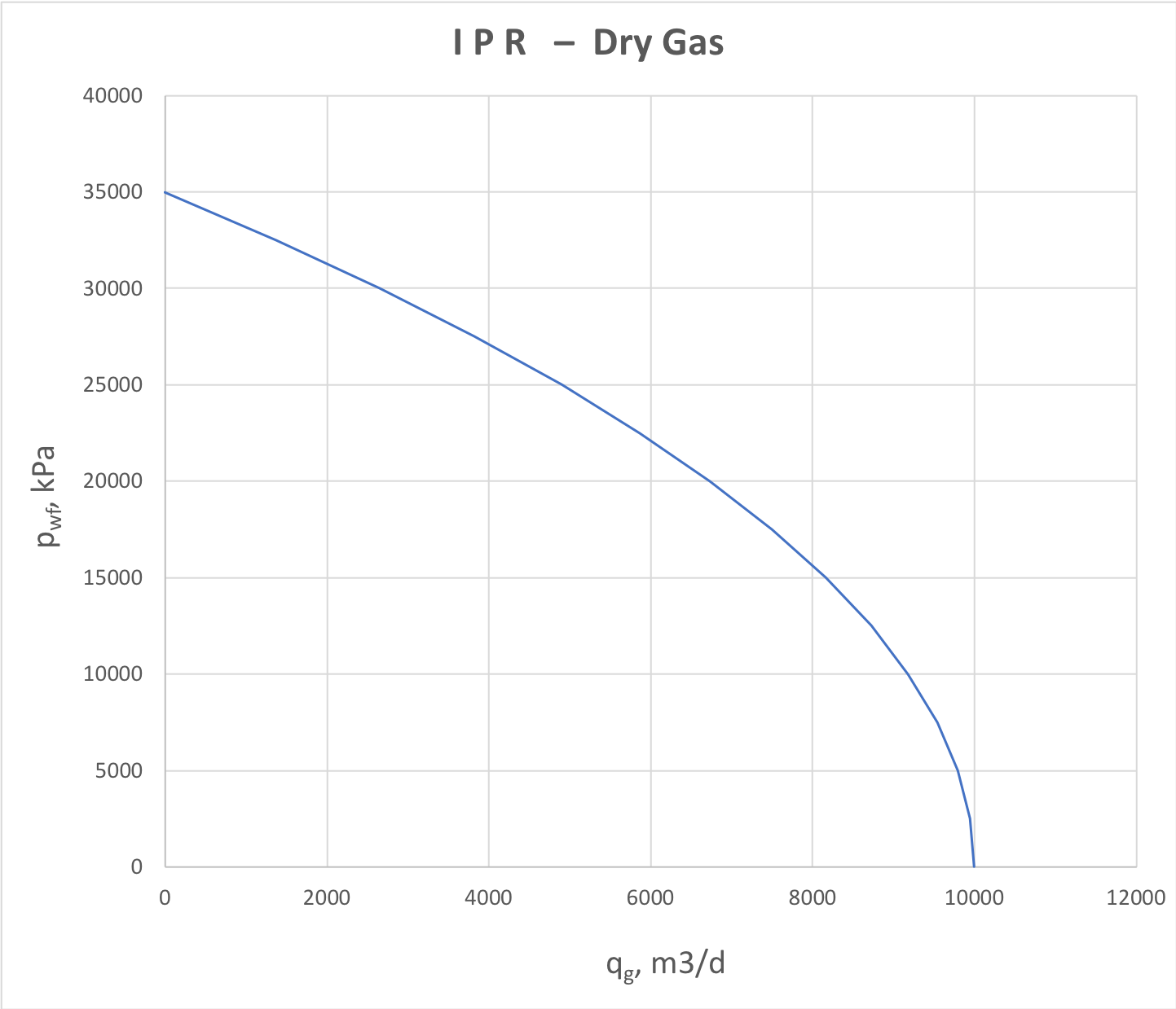
For gas producers, the fluid compressibility is high and formation flow is essentially non-linear, inflicting the downward trend on the whole IPR plot (Fig. 2).
|
Fig. 2. IPR for dry gas producer or gas injector into a gas formation |
The popular dry gas IPR correlation is Rawlins and Shellhardt:
| LaTeX Math Block |
|---|
| anchor | IPRGas |
|---|
| alignment | left |
|---|
|
\frac{q}{q_{max}} = \Bigg[ \, 1- \Bigg( \frac{p_{wf}}{p_Rr} \Bigg)^2 \, \Bigg]^n |
where
is the turbulent flow exponent, equal to 0.5 for fully turbulent flow and equal to 1 for laminar flow.
The more accurate approximation is given by LIT (Laminar Inertial Turbulent) IPR model:
| LaTeX Math Block |
|---|
|
a \, q + b \, q^2 = \Psi(p_r) - \Psi(p_{wf}) |
where
– is pseudo-pressure function specific to a certain gas PVT model,
is laminar flow coefficient and
is turbulent flow coefficient.
It needs two well tests at two different rates to assess
| LaTeX Math Inline |
|---|
| body | \{ q_{max} \, , \, n \} |
|---|
|
or
.
But obviously more tests will make assessment more accruate.
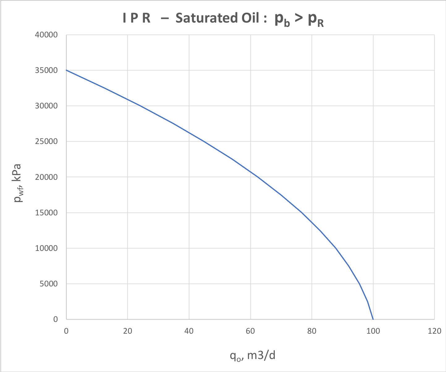
For saturated oil reservoir the free gas flow inflict the downward trend of IPR plot similar to dry gas (Fig. 3).
|
Fig. 3. IPR for 2-phase oil+gas production below and above bubble point |
The analytical correlation for saturted oil flow is given by Vogel model:
| LaTeX Math Block |
|---|
|
\frac{q}{q_{max}} = 1 - 0.2 \, \frac{p_{wf}}{p_r} - 0.8 \Bigg(\frac{p_{wf}}{p_r} \Bigg)^2 \quad , \quad p_b > p_r > p_{wf} |
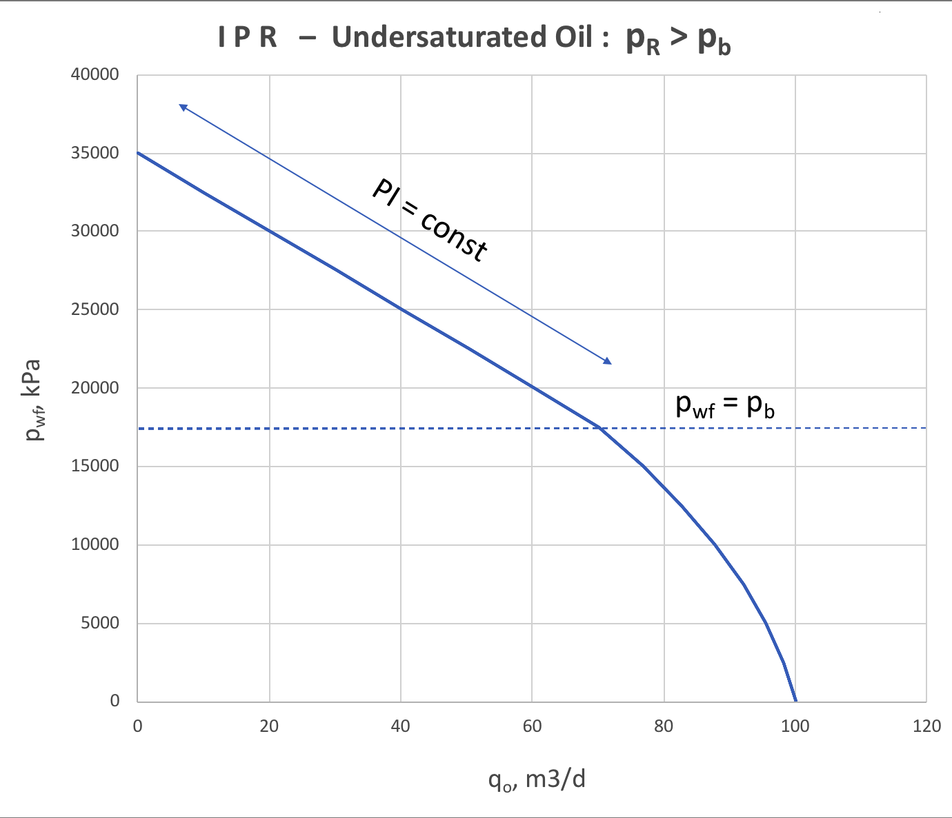
For undersaturated oil reservoir
the behavior of
IPR model will vary on whether the bottom-hole pressure is above or below bubble point.
When it is higher than bubble point
then formation flow will be single-phase oil and production will follow the constant
IPR (Inflow Performance Relation).
When bottom-hole pressure goes below bubble point
the near-reservoir zone free gas slippage also inflicts the downward trend at the right side of
IPR plot (Fig. 3).
It can be interpreted as deterioration of near-reservoir zone permeability when the fluid velocity is high and approximated by rate-dependant skin-factor.
|
Fig. 3. IPR for 2-phase oil+gas production below and above bubble point |
The analytical correlation for undersaturated oil flow is given by modified Vogel model:
| LaTeX Math Block |
|---|
|
\frac{q}{q_b} = \frac{p_r - p_{wf}}{p_r - p_b} \quad , \quad p_r > p_{wf} > p_b |
| LaTeX Math Block |
|---|
| anchor | ModifiedVogel |
|---|
| alignment | left |
|---|
|
q = (q_{max} - q_b ) \Bigg[ 1 - 0.2 \, \frac{p_{wf}}{p_b} - 0.8 \Bigg(\frac{p_{wf}}{p_b} \Bigg)^2 \Bigg] + q_b \quad , \quad p_r > p_b > p_{wf} |
with AOF
related to bubble point flowrate
via following correlation:
| LaTeX Math Block |
|---|
|
q_{max} = q_b \, \Big[1 + \frac{1}{1.8} \frac{p_b}{(p_r - p_b)} \Big] |
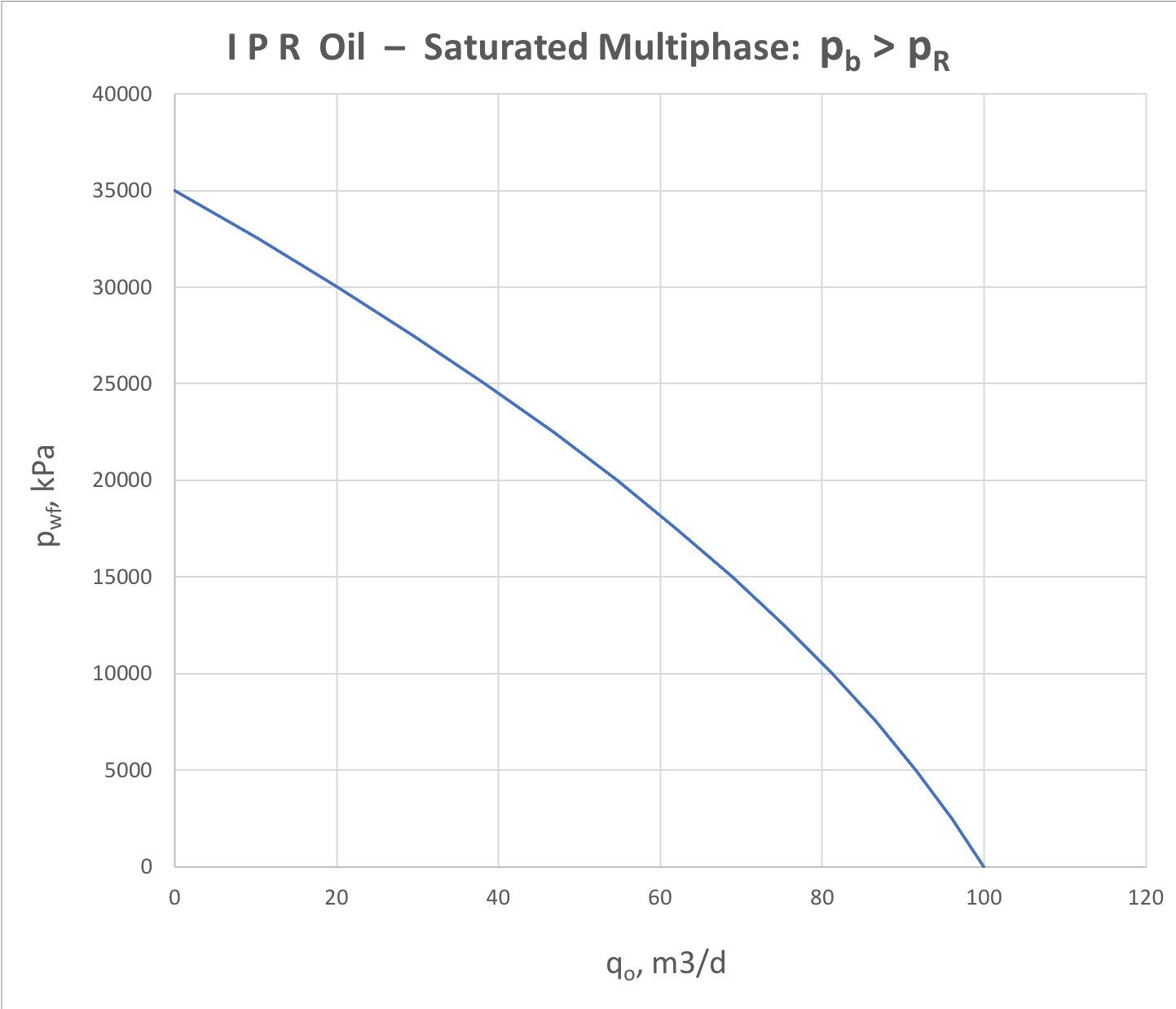
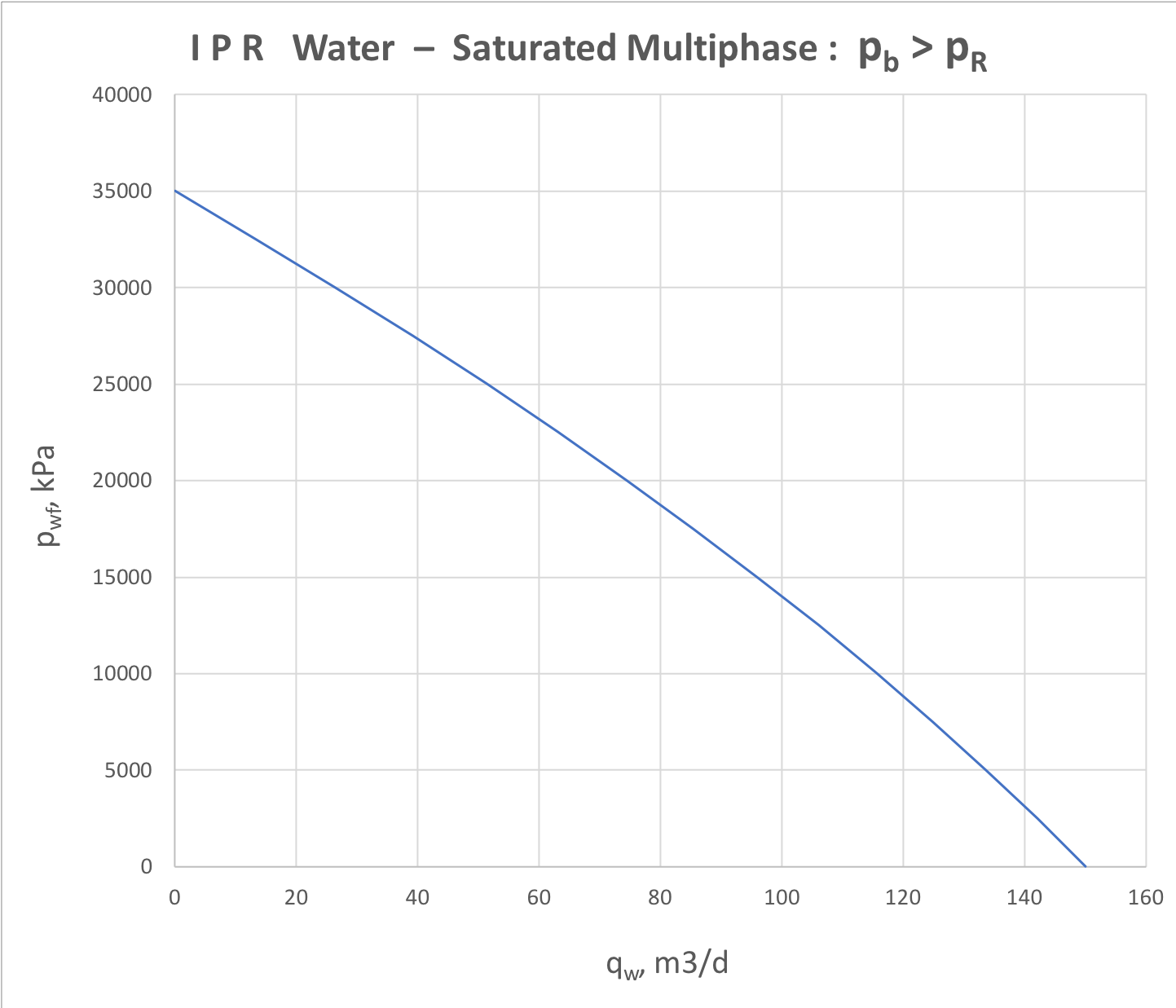
For saturated 3-phase water-oil-gas reservoir the IPR analysis is represented by oil and water components separately (see Fig. 4.1 and Fig. 4.2).
| |
Fig. 4.1. Oil IPR for saturated 3-phase (water + oil + gas) formation flow | Fig. 4.2. Water IPR for saturated 3-phase (water + oil + gas) formation flow |
The analytical correlation for saturated 3-phase oil flow is given by Wiggins model:
| LaTeX Math Block |
|---|
|
\frac{q_o}{q_{o, \, max}} = 1 - 0.52 \, \frac{p_{wf}}{p_r} - 0.48 \Bigg(\frac{p_{wf}}{p_r} \Bigg)^2 |
| LaTeX Math Block |
|---|
|
\frac{q_w}{q_{w, \, max}} = 1 - 0.72 \, \frac{p_{wf}}{p_r} - 0.28 \Bigg(\frac{p_{wf}}{p_r} \Bigg)^2 |
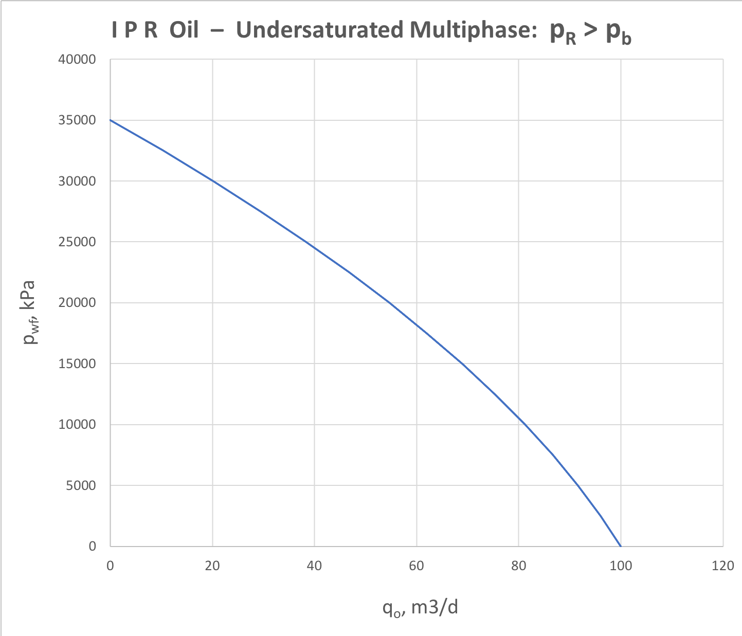
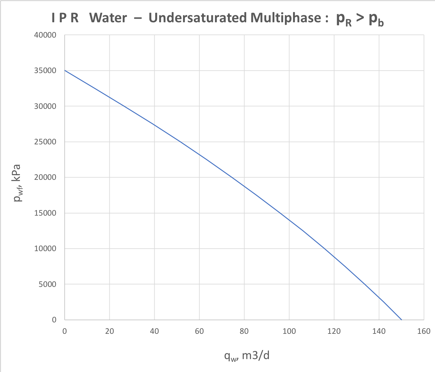
For undersaturated 3-phase water-oil-gas reservoir the IPR analysis is represented by oil and water components separately (see Fig. 4.1 and Fig. 4.2).
| |
Fig. 4.1. Oil IPR for udersaturated 3-phase (water + oil + gas) formation flow | Fig. 4.2. Water IPR for undersaturated 3-phase (water + oil + gas) formation flow |