Consider a system of net hydrocarbon pay and finite or infinite volume Aquifer as a radial composite reservoir with inner composite area being a Net Pay Area and outer composite area an Aquifer
(see schematic and notations on Fig. 1 at Radial VEH Aquifer Drive @model).
The Aquifer's outer boundary may be "no-flow" for finite-volume Aquifer or constant pressure for infinite-volume Aquifer.
The transient pressure diffusion in the outer (Aquifer) composite area is going to honour the following equation:
| Driving equation | Initial condition |
|
|---|
Homogeneous Aquifer reservoir with | Initial Aquifer pressure is considered to be the same as Net Pay Area |
...
| borderColor | wheat |
|---|
| borderWidth | 10 |
|---|
123
...
|
|
| LaTeX Math Block |
|---|
| \frac{\partial p_a}{\partial t} = \chi \cdot \left[ \frac{\partial^2 p_a}{\partial r^2} + \frac{1}{r}\cdot \frac{\partial p_a}{\partial r} \right] |
| | LaTeX Math Block |
|---|
| p_a(t = 0, r)= p(0) |
| |
| Inner Aquifer boundary | Outer Aquifer boundary is one of the two below: |
|---|
| Pressure variation at the contact with Net Pay Are | "No-flow" | "Constant pressure" |
| LaTeX Math Block |
|---|
| p_a(t, r=r_e) = p(t) |
| |
...
| \frac{\partial p_a}{\partial r}
\bigg|_{(t, r=r_a)} = 0 |
| | LaTeX Math Block |
|---|
| anchor | pconst |
|---|
| alignment | left |
|---|
| p_a(t, r = \infty) = 0 |
|
Consider
...
dimensionless solution
of the following equation:| LaTeX Math Block |
|---|
| \frac{\partial p_1}{\partial t_D} = \frac{\partial^2 p_1}{\partial r_D^2} + \frac{1}{r_D}\cdot \frac{\partial p_1}{\partial r_D} |
| | LaTeX Math Block |
|---|
| p_1(t_D = 0, r_D)= 0 |
| | LaTeX Math Block |
|---|
| p_1(t_D, r_D=1) = 1 |
| | LaTeX Math Block |
|---|
| \frac{\partial p_1(t_D, r_D)}{\partial r_D}
\Bigg|_{r_D=r_{aD}} = 0 \quad {\rm or} \quad p_1(t_D, r_D = \infty) = 0 |
|
which represents a unique function of dimensionless time
and distance .
Now consider a convolution integral:
| LaTeX Math Block |
|---|
| p_a(t, r) = p(0) + \int_0^t p_1 \left(\frac{(t-\tau) \cdot \chi}{r_e^2}, \frac{r}{r_e} \right) \dot p(\tau) d\tau |
| | LaTeX Math Block |
|---|
| \dot p(\tau) = \frac{d p}{d \tau} |
|
One can easily check that
| LaTeX Math Block Reference |
|---|
|
...
honours the whole set of equations
| LaTeX Math Block Reference |
|---|
|
–| LaTeX Math Block Reference |
|---|
|
...
/| LaTeX Math Block Reference |
|---|
|
and as such defines a unique solution of the above problem....
Now having the pressure dynamics in hand one can calculate the water influx.
The water flowrate within
sector angle at the interface with ...
net pay is:
| LaTeX Math Block |
|---|
| 1 |
q^{\downarrow}_{AQ}(t)= \theta \cdot r_e \cdot h \cdot u(t,r_e) |
where
is flow velocity at ...
Net Pay ↔ Aquifer contact boundary, which is:
| LaTeX Math Block |
|---|
| 1 |
u(t,r_e) = M \cdot \frac{\partial p_a(t,r)}{\partial r} \bigg|_{r=r_e} |
where
| LaTeX Math Inline |
|---|
| body | --uriencoded--\displaystyle M = \frac%7Bk_w%7D%7B\mu_w%7D |
|---|
|
is ...
Aquifer mobility.
...
The water flowrate is going to be:
| LaTeX Math Block |
|---|
| 1 |
q^{\downarrow}_{AQ}(t)= \theta \cdot r_e \cdot h \cdot M \cdot \frac{\partial p_a(t,r)}{\partial r} \bigg|_{r=r_e}Cumulative |
and cumulative water flux is going to be:
| LaTeX Math Block |
|---|
|
Q^{\downarrow}_{AQ}(t) = \int_0^t q^{\downarrow}_{AQ}(t) dt = \theta \cdot r_e \cdot h \cdot M \cdot \int_0^t \frac{\partial p_a(t,r)}{\partial r} \bigg|_{r=r_e} dt |
Substituting
| LaTeX Math Block Reference |
|---|
|
into | LaTeX Math Block Reference |
|---|
|
leads to:| LaTeX Math Block |
|---|
|
Q^{\downarrow}_{AQ}(t) = \theta  \cdot r_e \cdot h \cdot M  \cdot \int_0^t d\xi \  \frac{\partial }{\partial r} \left[

\int_0^\xi p_1 \left( \frac{(\xi-\tau)\chi}{r_e^2}, \frac{r}{r_e} \right) \, \dot p(\tau) d\tau

\right]_{r=r_e} |
| LaTeX Math Block |
|---|
| 1 |
Q^{\downarrow}_{AQ}(t) = \theta  \cdot h \cdot M  \cdot \int_0^t d\xi \  \frac{\partial }{\partial r_D} \left[

\int_0^\xi p_1 \left( \frac{(\xi-\tau)\chi}{r_e^2}, r_D \right) \, \dot p(\tau) d\tau

\right]_{r_D=1} |
| LaTeX Math Block |
|---|
| 1 |
Q^{\downarrow}_{AQ}(t) = \theta  \cdot h \cdot M  \cdot \int_0^t d\xi \

\int_0^\xi \frac{\partial p_1}{\partial r_D} \left( \frac{(\xi-\tau)\chi}{r_e^2}, r_D \right) \Bigg|_{r_D=1} \, \dot p(\tau) d\tau
|
The above integral represents the integration over the
area in plane (see Fig. 1):| LaTeX Math Block |
|---|
| 1 |
Q^{\downarrow}_{AQ}(t) = \theta  \cdot h \cdot M  \cdot \iint_D d\xi \ d\tau  \, \dot p(\tau)

\frac{\partial p_1}{\partial r_D} \left( \frac{(\xi-\tau)\chi}{r_e^2}, r_D \right) \Bigg|_{r_D=1}
|
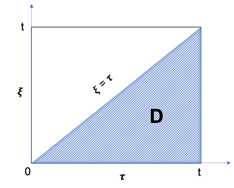 Image Modified Image Modified
|
Fig. 1. Illustration of the integration area in plane |
Changing the integration order from
to leads to:| LaTeX Math Block |
|---|
| 1 |
Q^{\downarrow}_{AQ}(t) = \theta  \cdot h \cdot M  \cdot \int_0^t d\tau \int_\tau^t d\xi  \ \dot p(\tau)

\frac{\partial p_1}{\partial r_D} \left( \frac{(\xi-\tau)\chi}{r_e^2}, r_D \right) \Bigg|_{r_D=1}
=
 \theta  \cdot h \cdot M  \cdot \int_0^t \dot p(\tau) d\tau \int_\tau^t d\xi  \

\frac{\partial p_1}{\partial r_D} \left( \frac{(\xi-\tau)\chi}{r_e^2}, r_D \right) \Bigg|_{r_D=1} |
Replacing the variable:
| LaTeX Math Block |
|---|
| 1 |
\xi = \tau + \frac{r_e^2}{\chi} \cdot t_D \rightarrow t_D = \frac{(\xi-\tau)\chi}{r_e^2} \rightarrow d\xi = \frac{r_e^2}{\chi} \cdot dt_D |
and
...
cumulative influx becomes:
| LaTeX Math Block |
|---|
| 1 |
Q^{\downarrow}_{AQ}(t) = \theta  \cdot h \cdot M \cdot \frac{r_e^2}{\chi} \cdot \int_0^t \dot p(\tau) d\tau \int_0^{(t-\tau)\chi/r_e^2}

\frac{\partial p_1( t_D, r_D)}{\partial r_D}  \Bigg|_{r_D=1} dt_D = B \cdot \int_0^t \dot p(\tau) d\tau \int_0^{(t-\tau)\chi/r_e^2}

\frac{\partial p_1( t_D, r_D)}{\partial r_D} \Bigg|_{r_D=1} dt_D |
where
is water influx constant and which leads to:| LaTeX Math Block |
|---|
-ref |
|---|
| and | LaTeX Math Block Reference |
|---|
|
.qwe |
Q^{\downarrow}_{AQ}= B \cdot \int_0^t W_{eD} \left( \frac{(t-\tau)\chi}{r_e^2}\right) \dot p(\tau) d\tau |
where
| LaTeX Math Block |
|---|
|
W_{eD}(t) = \int_0^{t} \frac{\partial p_1}{\partial r_D} \bigg|_{r_D = 1} dt_D |
is a unique dimensionless function of dimensionless time
which can be tabulated via numerical solution or approximated by closed-form expression.
See Also
...
Petroleum Industry / Upstream / Subsurface E&P Disciplines / Field Study & Modelling / Aquifer Drive / Aquifer Drive Models / Radial VEH Aquifer Drive @model