Motivation
| Excerpt Include |
|---|
| Aquifer Drive |
|---|
| Aquifer Drive |
|---|
| nopanel | true |
|---|
|
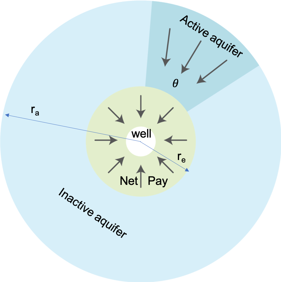
Physical Model
Mathematical Model
| LaTeX Math Block |
|---|
| Q^{\downarrow}_{AQ}= B \cdot \int_0^t W_{eD} \left( \frac{(t-\tau)\chi_a}{r_e^2} \right) \dot p(\tau) d\tau |
|
| LaTeX Math Block |
|---|
| q^{\downarrow}_{AQ}(t)= \frac{dQ^{\downarrow}_{AQ}}{dt} |
|
| LaTeX Math Block |
|---|
| W_{eD}(t)= \int_0^{t} \frac{\partial p_1}{\partial r_D} \bigg|_{r_D = 1} dt_D |
| |
| LaTeX Math Block |
|---|
| \frac{\partial p_1}{\partial t_D} = \frac{\partial^2 p_1}{\partial r_D^2} + \frac{1}{r_D}\cdot \frac{\partial p_1}{\partial r_D} |
|
| LaTeX Math Block |
|---|
| p_1(t_D = 0, r_D)= 0 |
|
| LaTeX Math Block |
|---|
| p_1(t_D, r_D=1) = 1 |
|
| LaTeX Math Block |
|---|
| \frac{\partial p_1}{\partial r_D}
\bigg|_{(t_D, r_D=r_a/r_e)} = 0 |
|
| Expand |
|---|
|
| Panel |
|---|
|
Transient flow in Radial Composite Reservoir:
| LaTeX Math Block |
|---|
| \frac{\partial p_a}{\partial t} = \chi \cdot \left[ \frac{\partial^2 p_a}{\partial r^2} + \frac{1}{r}\cdot \frac{\partial p_a}{\partial r} \right] |
|
| LaTeX Math Block |
|---|
| p_a(t = 0, r)= p(0) |
|
| LaTeX Math Block |
|---|
| p_a(t, r=r_e) = p(t) |
|
| LaTeX Math Block |
|---|
| anchor | p1_PSS |
|---|
| alignment | left |
|---|
| \frac{\partial p_a}{\partial r}
\bigg|_{(t, r=r_a)} = 0 |
|
Consider a pressure convolution:
| LaTeX Math Block |
|---|
| p_a(t, r) = p(0) + \int_0^t p_1 \left(\frac{(t-\tau) \cdot \chi_a}{r_e^2}, \frac{r}{r_e} \right) \dot p(\tau) d\tau |
|
| LaTeX Math Block |
|---|
| \dot p(\tau) = \frac{d p}{d \tau} |
|
One can easily check that | LaTeX Math Block Reference |
|---|
|
honors the whole set of equations | LaTeX Math Block Reference |
|---|
|
–| LaTeX Math Block Reference |
|---|
|
and as such defines a unique solution of the above problem.Water flowrate within sector angle at interface with oil reservoir will be:| LaTeX Math Block |
|---|
| q^{\downarrow}_{AQ}(t)= \theta \cdot r_e \cdot h_a \cdot u(t,r_e) |
where is flow velocity at aquifer contact boundary, which is:| LaTeX Math Block |
|---|
| u(t,r_e) = M_a \cdot \frac{\partial p_a(t,r)}{\partial r} \bigg|_{r=r_e} |
where | LaTeX Math Inline |
|---|
| body | M_a = \frac{k_a}{\mu_w} |
|---|
|
is aquifer mobility.Water flowrate becomes: | LaTeX Math Block |
|---|
| q^{\downarrow}_{AQ}(t)= \theta \cdot r_e \cdot h_a \cdot M_a \cdot \frac{\partial p_a(t,r)}{\partial r} \bigg|_{r=r_e} |
Cumulative water flux: | LaTeX Math Block |
|---|
| Q^{\downarrow}_{AQ}(t) = \int_0^t q^{\downarrow}_{AQ}(t) dt = \theta \cdot r_e \cdot h_a \cdot M_a \cdot \int_0^t \frac{\partial p_a(t,r)}{\partial r} \bigg|_{r=r_e} dt |
Substituting | LaTeX Math Block Reference |
|---|
|
into | LaTeX Math Block Reference |
|---|
|
leads to:| LaTeX Math Block |
|---|
| Q^{\downarrow}_{AQ}(t) = \theta \cdot r_e \cdot h_a \cdot M_a \cdot \int_0^t d\xi \ \frac{\partial }{\partial r} \left[
\int_0^\xi p_1 \left( \frac{(\xi-\tau)\chi_a}{r_e^2}, \frac{r}{r_e} \right) \, \dot p(\tau) d\tau
\right]_{r=r_e} |
| LaTeX Math Block |
|---|
| Q^{\downarrow}_{AQ}(t) = \theta \cdot h_a \cdot M_a \cdot \int_0^t d\xi \ \frac{\partial }{\partial r_D} \left[
\int_0^\xi p_1 \left( \frac{(\xi-\tau)\chi_a}{r_e^2}, r_D \right) \, \dot p(\tau) d\tau
\right]_{r_D=1} |
| LaTeX Math Block |
|---|
| Q^{\downarrow}_{AQ}(t) = \theta \cdot h_a \cdot M_a \cdot \int_0^t d\xi \
\int_0^\xi \frac{\partial p_1}{\partial r_D} \left( \frac{(\xi-\tau)\chi_a}{r_e^2}, r_D \right) \Bigg|_{r_D=1} \, \dot p(\tau) d\tau
|
The above integral represents the integration over the area in plane (see Fig. 1):| LaTeX Math Block |
|---|
| Q^{\downarrow}_{AQ}(t) = \theta \cdot h_a \cdot M_a \cdot \iint_D d\xi \ d\tau \, \dot p(\tau)
\frac{\partial p_1}{\partial r_D} \left( \frac{(\xi-\tau)\chi_a}{r_e^2}, r_D \right) \Bigg|_{r_D=1}
|
| Fig. 1. Illustration of the integration area in plane |
Changing the integration order from to leads to:| LaTeX Math Block |
|---|
| Q^{\downarrow}_{AQ}(t) = \theta \cdot h_a \cdot M_a \cdot \int_0^t d\tau \int_\tau^t d\xi \ \dot p(\tau)
\frac{\partial p_1}{\partial r_D} \left( \frac{(\xi-\tau)\chi_a}{r_e^2}, r_D \right) \Bigg|_{r_D=1}
=
\theta \cdot h_a \cdot M_a \cdot \int_0^t \dot p(\tau) d\tau \int_\tau^t d\xi \
\frac{\partial p_1}{\partial r_D} \left( \frac{(\xi-\tau)\chi_a}{r_e^2}, r_D \right) \Bigg|_{r_D=1} |
Replacing the variable: | LaTeX Math Block |
|---|
| \xi = \tau + \frac{r_e^2}{\chi_a} \cdot t_D \rightarrow t_D = \frac{(\xi-\tau)\chi_a}{r_e^2} \rightarrow d\xi = \frac{r_e^2}{\chi_a} \cdot dt_D |
and flux becomes: | LaTeX Math Block |
|---|
| Q^{\downarrow}_{AQ}(t) = \theta \cdot h_a \cdot M_a \cdot \frac{r_e^2}{\chi_a} \cdot \int_0^t \dot p(\tau) d\tau \int_0^{(t-\tau)\chi_a/r_e^2}
\frac{\partial p_1( t_D, r_D)}{\partial r_D} \Bigg|_{r_D=1} dt_D |
and finally: | LaTeX Math Block |
|---|
| Q^{\downarrow}_{AQ}(t) = \theta \cdot h_a \cdot M_a \cdot \frac{r_e^2}{\chi_a} \cdot \int_0^t \dot p(\tau) d\tau \int_0^{(t-\tau)\chi_a/r_e^2}
\frac{\partial p_1( t_D, r_D)}{\partial r_D} \Bigg|_{r_D=1} dt_D |
which leads to | LaTeX Math Block Reference |
|---|
|
and | LaTeX Math Block Reference |
|---|
|
. |
|
See Also
Petroleum Industry / Upstream / Subsurface E&P Disciplines / Field Study & Modelling / Aquifer Drive / Aquifer Drive Models
Reference
1. van Everdingen, A.F. and Hurst, W. 1949. The Application of the Laplace Transformation to Flow Problems in Reservoirs. Trans., AIME 186, 305.
2. Tarek Ahmed, Paul McKinney, Advanced Reservoir Engineering (eBook ISBN: 9780080498836)
3. Klins, M.A., Bouchard, A.J., and Cable, C.L. 1988. A Polynomial Approach to the van Everdingen-Hurst Dimensionless Variables for Water Encroachment. SPE Res Eng 3 (1): 320-326. SPE-15433-PA. http://dx.doi.org/10.2118/15433-PA