1. Collect urface flowrates  and bottom-hole pressure (BHP)  which are normally available with permanent downhole gauges (PDG)
  2. Data filtering
    1. Filter the BHP  data for overshoots
    2. Filter the BHP data with wavelet thresholding to reduce the noise
    3. Decimate the BHP data (usually 10:1 or 100:1)
    4. Translate the Surface flowrates  to Total sandface flowrate   with account of BHP  at any moment of time
    5. Synchronise total flowrate qt variations with BHP variations
    6. Create multi-well history plot with qtBHP, Yw, GOR/Rs.
  3. Primary Analysis
    1. Filter out shut-ins and hold drawdowns only
    2. Create material balance (BHP and Pe vs cum Q) and IPR (BHP vs qt) diagnostic metrics over the drawdown history
    3. Identify the zones of constant productivity index (PI = const), Steady-states (SS) and pseudo steady-states (PSS)
    4. Assess dynamic drainage volume Ve for all wells – this is a volume which well is currently draining with account of interference with other wells
  4. Deconvolution
    1. Select the constant Productivity Index time segments
    2. Remove pressure data during shut-in periods except possibly few valuable (representative and similar to drawdown)
    3. Process PBUs to assess formation pressures
    4. Input formation pressure Pe as constrains for future deconvolution
    5. Tune up the weights to match deconvolution trials with PBUs against DTRs
    6. In case of wells are sitting in the same homogenous reservoir compartment with no behind-casing complications then assume CTR are symmetric to further constrain deconvolution
    7. Perform multiwell deconvolution and QC
    8. Analyse the response and separate wells by non-interfering groups
    9. Repeat multiwell deconvolution for each well group and each constant PI time period
  5. Convolution and analysis
    1. Reconstruct formation pressure Pe history
    2. Reconstruct productivity index history
    3. Validate if PI is constant and repeat deconvolution exercises over various time intervals if required
    4. Analyse rates correction and check if it is within the metrological limits and raise allocation concerns and/or advise the corrections
    5. Create unit-rate spider-plot – a pressure impact diagram showing how  one well with unit-rate would be varying the pressure in another well over time
    6. Create historical rates spider-plot – a pressure impact diagram showing how one well was varying the pressure in another well over time
    7. Create historical rates pressure interference map showing a current and cumulative impact from one well on another
    8. Create oil IPR at different formation pressure markups and analyse production optimisation potentials 
  6. Analytical modelling 
    1. Perform analytical pressure diffusion modelling of all DTR/CTR wit conventional Pressure Transient Analysis (PTA) using log-derivative log-log plots 
    2. Assess potential drainage volume Ve,max for all wells – the volumes which well would be draining in case it would be the inly producing well in the field
    3. Assess well drainage transmissibility and cross-well transmissibility and compare them against each other and against the OH  log interpretation on the map
    4. Analyse additional diffusion model parameters (skin-factor, fracture length, horizontal length, permeability anisotropy) against expectations
  7. Additional studies
    1. Production forecasts
      1. Generate formation pressure and bottom-hole pressure forecasts based on NFA production/injection rates
      2. Generate formation pressure and production forecasts based on constant BHP
      3. Additional forecasts based on various BHP and production scenarios
    2. Numerical pressure tests
      1. Create N2 numerical pressure test scenarios for each DTR and CTR
      2. Check  simulated DTR/CTR against deconvolved DTR/CTR in log-derivative diagnostic plots to understand where exactly numerical model may have discrepancies 
      3. Try various model boundaries, barriers and reservoir properties to improve the match

See Also


Petroleum Industry / Upstream /  Production / Subsurface Production / Field Study & Modelling / Production Analysis / Multiwell Retrospective Testing (MRT)


These days a lot of producing wells is equipped with permanent Downhole Gauges (PDG), particularly in ESP wells.

Given a fact the production rates are constantly changing for technical reasons this allows studying the PDG response to the interference with offset wells.

Despite of an obvious appeal this idea has a number of substantial drawbacks:


  1. Low sensitivity of most PDGs 
     
    It's usually around 15 psi with ability to be programmed for 1.5 psi which is still very poor for the purposes of corse-well interference analysis. 
    Besides most of PDG data today has been already recorded in 15 psi mode even though these Pigs allow 1.5 psi mode.

     
  2. Poor time-step in PDG readings

     
    It's normal practise to record PDG with hourly or even daily step which is too rough for pressure interference analysis
     
  3. Poor tracking at injecting wells


Very often injectors are equipped with line gauges before the choke and can not sense the small pressure variations at the well bottom.
In some case injection THP is set after choke and can respond to formation pressure variations – although  with much worse sensitivity than downhole gauges due to the damping factor of borehole fluid.


The efficient method to analyse the historical PDG recordings today is the multi-well Radial Deconvolution which is built around a rate and PDG history in producing well and production history in offset wells.


The results of the RDCV for N wells one gets N transient responses (TR):

  1. One Drawdown transient response (DTR) for the PDG well which characterises the pressure response of the PDG well to its own rate variation
     
  2. N – 1 cross-well transient responses (CTR) for the interval between PDG and each of the N –1 surrounding wells and which characterises the impact the surrounding wells provide on the formation pressure in PDG well


Due to a poor pressure readings the quality of TR will be poor as well and not often they can interpreted in terms of transmissibility and diffusivity.

Particularly it is very rare when this type of TR can reveal fracture development or skin-factor.

But nevertheless it is still capable to assess formation pressure in PDG well quite accurately.

Below is the moist of the reliable deliverables one can get from RDCV in popular cases:

  1. Formation pressure in PDG well at any time in the past

  2. Comparative contribution oif the surrouding wells to the formation pressure in PDG well

  3. Qualitative assesment of the future formation pressure dynamic in PDG well under the arbitrary rate scenario in surrounding wells (whether it will grow or decline or stay flat)
     
  4. Rate History correction of the PDG well  which can be sed in realшocstion for accurate full-field simulations.


This set of information represent a high value for reservoir engineers for daily planning and also valuable for simulation engineers for 3D model calibration.

The weakest point of RDCB is its inability to distinguish the contour button off two (or more) wells which were changing its rate synchronously (or did not change it at all) during the whole time of the PDG recordings. 

Case Study


Здесь напрашивается хороший пример по РДКВ на основе ТМС с добывающими и нагнетательными скважинами – бросьте картинки и я напишу текст. (https://www.arax.team/company/personal/user/20/tasks/task/view/8642/)

Fig.1. Pressure and Rate history at producing well OP-6

Должна быть картинка иллюстрирующая грубую запись давления ТМС, грубую запись нагнетательной скважины (https://www.arax.team/company/personal/user/20/tasks/task/view/8642/)

Fig. 2. Pressure and Rate history at injecting well  Wl4


Fig. 3. Cumulative Withdrawals at 01.05.17 (with underlying thikness map)

Fig. 4. Current Withdrawals at 01.05.17 (with underlying thinkness map)


Портянка (https://www.arax.team/company/personal/user/20/tasks/task/view/8642/)

Рис.5. Pressure and Rate history of well OP-6 и and rate history of surrounding wells.

ПХ (https://www.arax.team/company/personal/user/20/tasks/task/view/8642/)

Fig.6. DTR for OP-6 OP-6


Динамика пластового давления центральной скважины (https://www.arax.team/company/personal/user/20/tasks/task/view/8642/)

Fig. 7. Reconstruction of formation pressure history and delta pressure at well OP-6


Сравнительный вклад окружающих скважин в пластовое давление по центральной скважине (https://www.arax.team/company/personal/user/20/tasks/task/view/8642/)

Fig. 8. Impact from offset Wells on formation pressure in OP-6Fig. 9. Impact from offset Wells on formation pressure in OP-6 (zoom)

Коррекция дебитов по центральной скважине – зум вокруг явной ошиьки в исторической записи (https://www.arax.team/company/personal/user/20/tasks/task/view/8642/)


Рис. 9. Rate correction at well  OP-6 


На сегодняшний день большая часть добывающего фонда с ЭЦН оборудованна системой погружной телеметрии (ТМС), которая, в частности, включает в себя датчик давления на входе в насос.

Учитывая, что режимы скважин постоянно меняются в силу технологических обстоятельств, это делает возможным анализ реакции датчика давления ТМС с целью оценки интерференции с окружающими скважинами.

Несмотря на видимую привлекательность, на этом пути есть серьезные практически ограничения:

  1. Низкая чувствительность датчика давления ТМС.

    Как правило чувствительность составляет 1 атм, и даже если возможность перевести его в режим 0.01 атм – это все-равно низкая чувствительность для амбициозных целей гидропрослушивания, к тому же исторические данные как правило записаны с чувствительностью 1 атм, даже если он поддерживает режим 0.01 атм – именно с этим приходиться иметь дело на практике.

  2. Грубый шаг записи датчика давления по времени.

    Зачастую данные пишутся несколько раз в сутки, а часто и один раз в сутки.

  3. Плохой контроль за давлением на нагнетательных скважинах 

    Иногда нагнетательные скважины оборудованы устьевыми манометрами на линии (до штуцера) и в этом случае информативность по реакции на окружение очень низкая.
    В случае если  нагнетательная скважина оборудована устьевым манометром на буфере (после штуцера), то  у него есть шансы отреагировать на смену режимов окружающих скважин и применить МДКВ, хотя чувствительность такого датчика будет хуже, чем у погружного из-за демпфирующего влияния ствола. 

Таким образом, наиболее подходящим методом анализа исторических данных по ТМС является радиальная деконволюция (РДКВ) вокруг добывающей скважины (по которой известна длительная история дебитов и забойного давления) и окружающих ее добывающих и нагнетательных скважин, от которых принимается во внимание история дебитов и расходов.

По итогам применения РДКВ к N скважинам получается N переходных характеристик (ПХ) :

  1. Одна диагональная для центральной скважины ТМС, которая характеризует влияния смены режимов центральной скважины на ее собственное забойной давление
     
  2.  N-1 кросс-диагональных ПХ в направлении окружающих ее скважин, которые характеризуют влияние смены режимов окружающих скважин на пластовое давление в центральной скважины


В силу низкого качества данных по давлению, качество ПХ будет тоже низким. 

Очень часто это не позволяет анализировать ранние и средние времена диагонального элемента на предмет оценки влияния трещины, аккуратных оценок скин-фактора и гидропроводности.

Однако оценка пластового давления и поздних времен может оказаться весьма успешной.

Вот список параметров которые можно получить на основе РДКВ по типовым скважинам с ТМС:

  1. Пластовое давление по центральной скважине на произвольный момент времени (этот параметр устойчив к неточностям диффузионной модели)

  2. Сравнительный вклад окружающих скважин в динамику пластового давления центральной скважины (кто влияет на центральную скважину больше, а кто меньше)

  3. Качественная оценка динамики пластового давления в районе центральной скважины и ее окружения под влиянием внешних (не входящих в РДКВ тест) окружающих скважин (либо тенденция к истощению, либо тенденция к полной компенсации и выходу на стационар, либо отсутствие влияния внешнего окружения)
     
  4. Коррекция дебита центральной скважины (что может использоваться при реаллокации данных по ГЗУ)


Эта информация представляет собой большую ценность для оперативного анализа разработки, а также может использоваться для калибровки 3Д моделей.

Необходимо помнить, что помимо качества исходной информации методы МДКВ имеют и естественные ограничения по информативности, в случае если режимы скважин менялись слабо и редко. 


Пример


Здесь напрашивается хороший пример по РДКВ на основе ТМС с добывающими и нагнетательными скважинами – бросьте картинки и я напишу текст. (https://www.arax.team/company/personal/user/20/tasks/task/view/8642/)

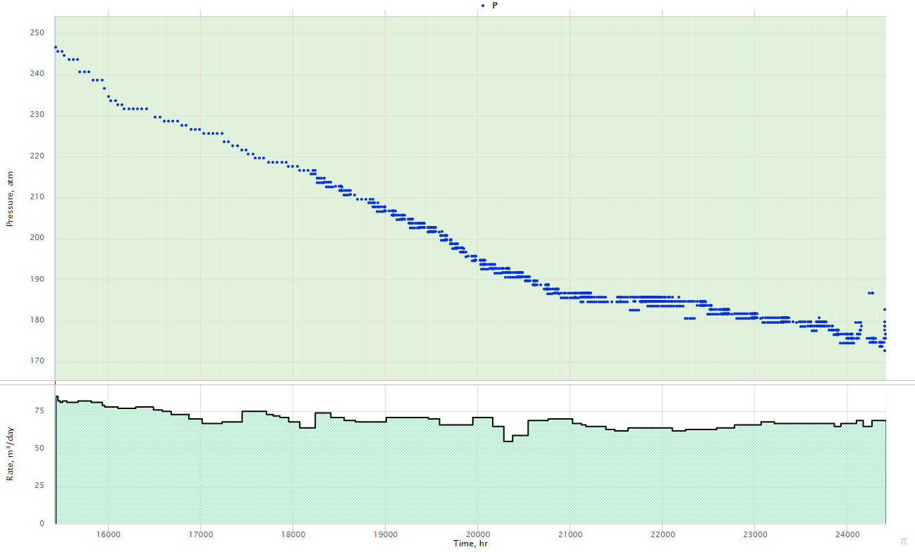
Рис.1. Запись давления ТМС и дебитов скважины OP-6

Должна быть картинка иллюстрирующая грубую запись давления ТМС, грубую запись нагнетательной скважины (https://www.arax.team/company/personal/user/20/tasks/task/view/8642/)

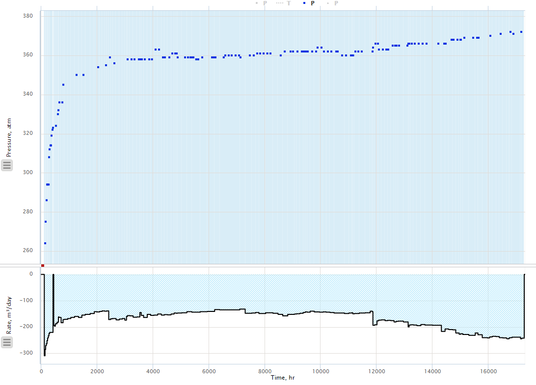
Рис.2. Запись давления  и дебитов скважины Wl4

Карта с накопленными и текущими отборами (https://www.arax.team/company/personal/user/20/tasks/task/view/8642/)

Рис.3. Карта накопленных отборов на 01.05.17 (подложка - карта толщин)

Рис.4. Карта текущих отборов на 01.05.17 (подложка - карта толщин)
Портянка (https://www.arax.team/company/personal/user/20/tasks/task/view/8642/)

Рис.5. Дебиты и давления скважины OP-6 и дебиты окружающих скважин.

ПХ (https://www.arax.team/company/personal/user/20/tasks/task/view/8642/)

Рис.6. Переходная Характеристика РДКВ OP-6 OP-6


Динамика пластового давления центральной скважины (https://www.arax.team/company/personal/user/20/tasks/task/view/8642/)

Рис. 7. Реконструкция пластового давления и депрессии на пласт в скважине OP-6


Сравнительный вклад окружающих скважин в пластовое давление по центральной скважине (https://www.arax.team/company/personal/user/20/tasks/task/view/8642/)

Рис. 8. График изменения пластового давления в зависимости от влияния соседних скважин на OP-6Рис. 9. График изменения пластового давления в зависимости от влияния соседних скважин на OP-6 (зум)

Коррекция дебитов по центральной скважине – зум вокруг явной ошиьки в исторической записи (https://www.arax.team/company/personal/user/20/tasks/task/view/8642/)


Рис. 9. График коррекции дебитов и давлений по РДКВ скважины OP-6