Inverse problem to pressure convolution, performed as a fully or semi-automated search for initial pressure for every well and Unit-rate Transient Responses (UTR) for wells and cross-well intervals in order to fit the sandface pressure response (usually recalculated from PDG data using wellbore flow model for depth adjustment ) to total sandface flow rate variation history (usually recalculated from daily allocations based on surface well tests). The basic element of deconvolution is the pressure Unit-rate Transient Response (UTR) which is a sandface pressure response to the total sandface unit-rate production. Multiwell deconvolution (MDCV) specifies two types of UTR: Drawdown Transient Response (DTR) and Cross-well Transient Response (CTR). The Drawdown Transient Response (DTR) is the sandface pressure response of a given well to its total sandface unit-rate production in absence of the other wells. It is equivalent to conventional Drawdown Test with sandface unit-rate production. The Cross-well Transient Response (CTR) is the sandface pressure response of a given well to the total sandface unit-rate production of the offset well in absence of the other wells. The pressure convolution principle itself has some limitations and may not be adequate for some practical cases. For example, changing reservoir conditions, high compressibility – everything which breaks linearity of diffusion equations. There are some workarounds on these cases but the best practice is to check the validity of pressure convolution (and therefore the applicability of MDCV) on the simple synthetic 2-well Dynamic Flow Model (DFM) with the typical for the given case reservoir-fluid-production conditions. MDCV can be performed in two options: Radial Deconvolution (
RDCV
) and Cross-well Deconvolution (
XDCV
). Radial Deconvolution (
RDCV
) correlates pressure and rate in selected well (called pressure-tested well) and only account for the rates in surrounding wells (called rate-tested wells) in order to reconstruct: A group of
N wells with one selected pressure-tested well has
N transient responses: 1 diagonal transient response and
N-1 cross-well transient responses. Only rates are taken into account for offset wells in RDCV. In case a group of tested wells have mulitple pressue gauge installations one may wish to deconvolve the unit-rate transient responses using all of the pressure data which is called Cross-well deconvolution (
XDCV
). The main advantage of
XDCV
over
RDCV
is the ability to simulate and interpret all PDG simultaneiously, resulting in mopre information and better constrain and stability of deconvolution process. The group of
N pressure-tested wells has
N^2 transient responses, because every well has 1 diagonal transient response and
N-1 cross-well transient responses thus having
N transient responses for each well. The intervals between two wells with pressure gauge instaltions results in two transient response: first well onto the second well and revers. This may indicate anisotropy of pressure propagation in counter directions and shed the light on the resevroir physics between these wells. Once all possible DTR/CTR are deconvolved one can perform a conventional type-curve analysis for each well, defining the type and distance to the boundary, estimating skin, transmissibility and diffusivity around each well. Unlike routine numericial fitting, where
N pressure responses to complicated rate history are being fit for
N wells, one can run XDCV to get
N^2 responses to very simple rate history (unit rate production) and then fit them all with diffusion models (sequentially or in parallel) by varying the same
4N parameters (current formation pressure around every well Pe, skin-factor S for every well, and usually, transmissibility σ + pressure diffusivity χ around each well). Main benefits of
MDCV
are: Main disadvantages of
MDCV
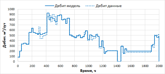
are: На рис. 2.1.2 представлена карта участка с тремя скважинами. Синтетическая история работы добывающей скважины с простым поведением продуктивности. Рис. 2.1.3. Скв. Р1. Сравнение мультискважинной деконволюции с односкважинной деконволюцией Рис. 2.1.4. P1. Сравнение полученной истории дебитов и давления с исходными На Рис. 2.1.5 представлена карта участка с тремя скважинами. Рис. 2.1.5. Синтетическая история работы добывающей скважины с простым поведением продуктивности Рис. 2.1.7. Влияние скважины P2 на скважину P1 Рис. 2.1.9. Скв. Р2. Сравнение мультискважинной деконволюции и односкважинной деконволюции На Рис. 2.1.15 приведена история дебитов и давлений по всем скважинам. Рис. 2.1.15. P1. Сравнение полученной истории дебитов и давления с исходнымиBasic concept
It is equivalent to the Pressure Interference Test with the unit-rate production in disturbing well.
The main difference between RDCV and single-well deconvolution (SDCV ) is that it takes into account offset wells impact on tested well pressure.Sample
Sample #1 – RDCV
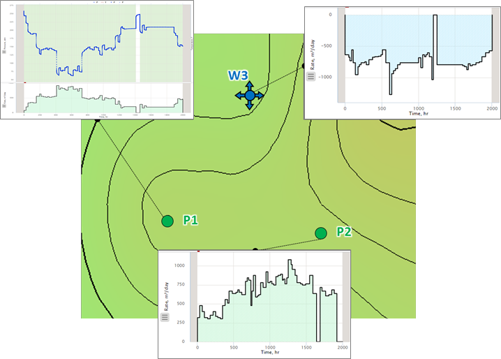
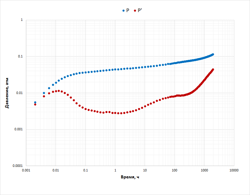
Рис. 2.1.2. Скв. Р1. Мультискважинная деконволюция 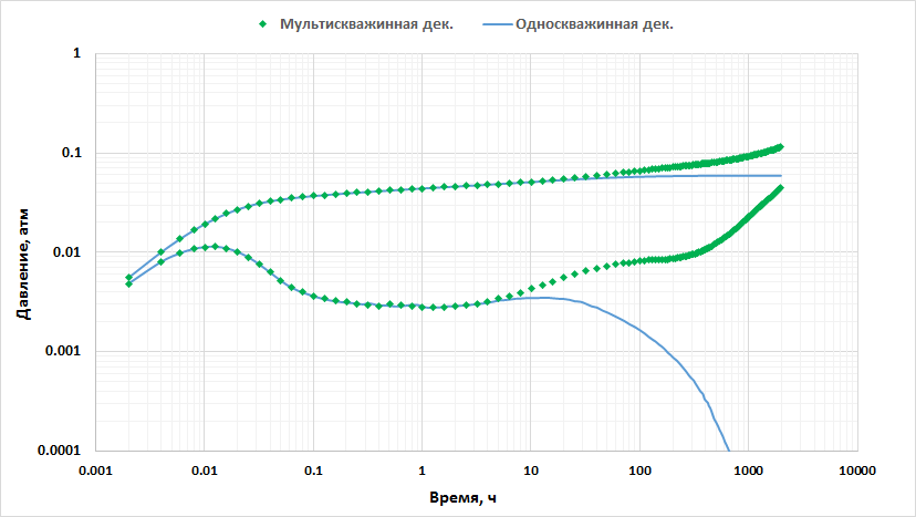
На Рис. 2.1.4 приведена история дебитов и давлений по всем скважинам.
Пример #2 – КДКВ
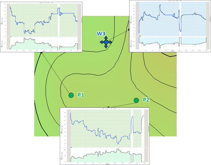
Рис. 2.1.6. Скв. Р1. Сравнение мультискважинной деконволюции и односкважинной деконволюции 
Рис. 2.1.8. Влияние скважины W3 на скважину P1 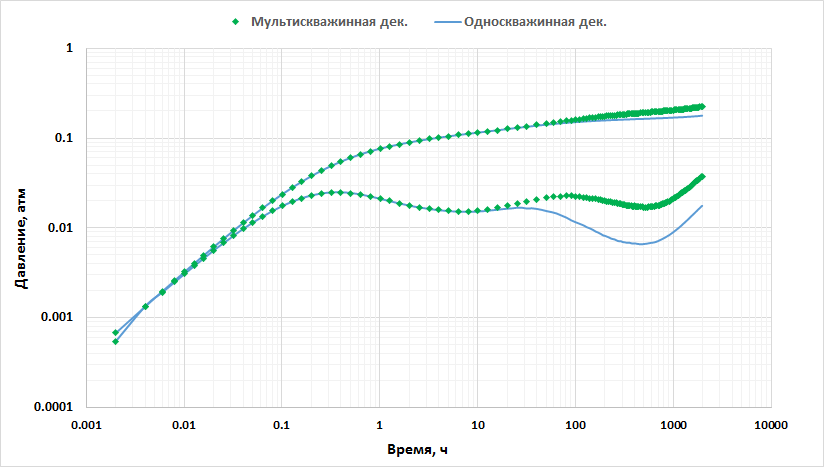
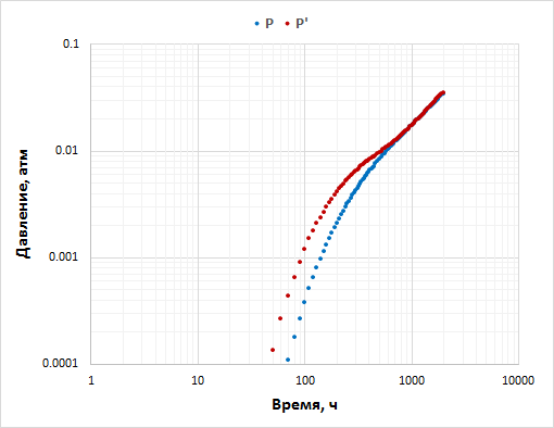
Рис. 2.1.10. Влияние скважины 1 на скважину 2 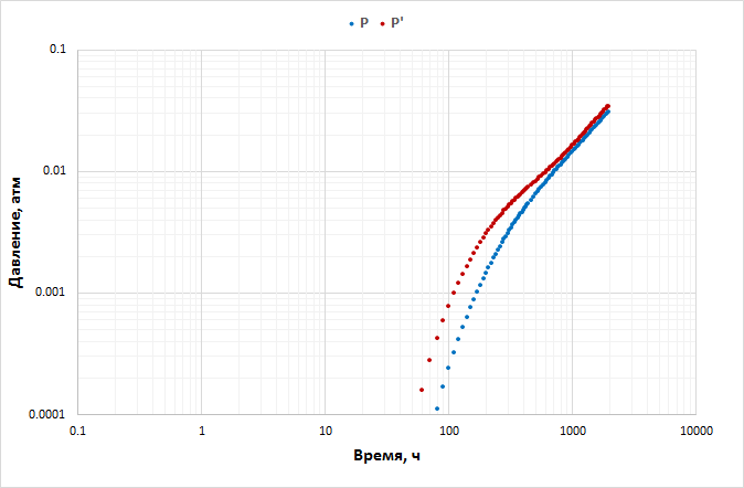
Рис. 2.1.11. Влияние скважины W3 на скважину P2 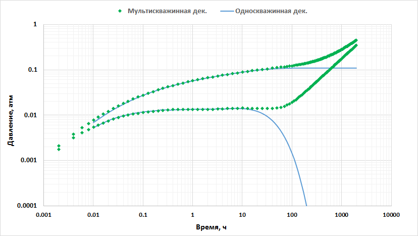
Рис. 2.1.12. Сравнение мультискважинной деконволюции и односкважинной деконволюции 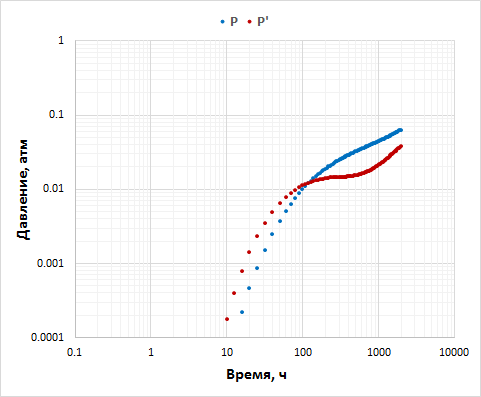
Рис. 2.1.13. Влияние скважины P1 на скважину W3 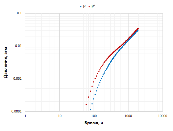
Рис. 2.1.14. Скв. W3 Влияние скважины P2 на скважину W3 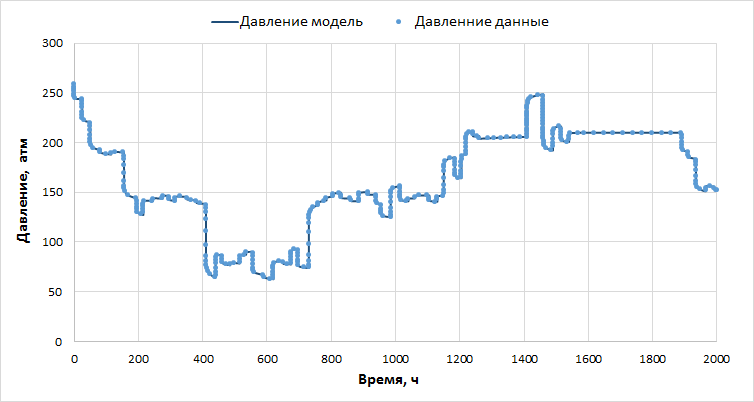

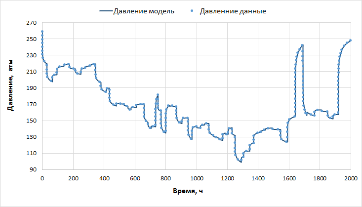
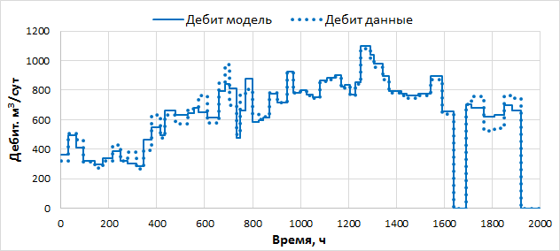
Рис. 2.1.16. P2. Сравнение полученной истории дебитов и давления с исходными 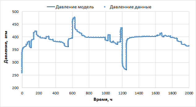
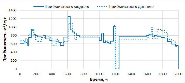
Рис. 2.1.17. W3. Сравнение полученной истории дебитов и давления с исходными
See Also
Petroleum Industry / Upstream / Subsurface E&P Disciplines / Well Testing / Pressure Testing / Pressure convolution / Pressure Deconvolution
[ MDCV @model ]