| Excerpt |
|---|
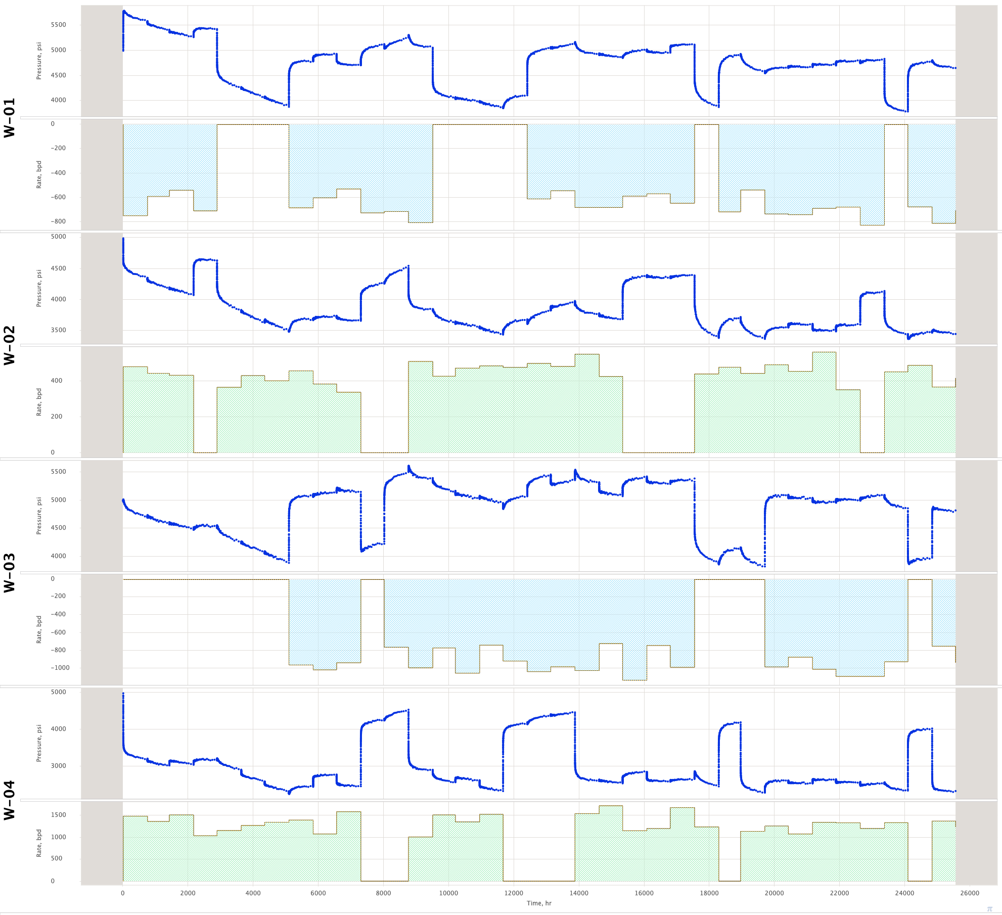
Inverse problem to pressure convolution, performed as a fully or semi-automated search for initial pressure for every well and unitUnit-rate transient responses Transient Responses (UTR) for wells and cross-well intervals in order to fit the sandface pressure response (usually recalculated from PDG data using wellbore flow model for depth adjustment adjustment) to total sandface flow rate variation history (usually recalculated from daily allocations based on surface well tests, see Fig. 1). | Expand |
|---|
|
|
| Column |
|---|
|
| Column |
|---|
|
Basic concept
The basic element of deconvolution is the pressure Transient Response (| Hint |
|---|
| 0 | TR |
|---|
| 1 | Transient Response |
|---|
| 2 | DTR |
|---|
|
) to a unit-rate flow.
| Hint |
|---|
| 0 | MDCV |
|---|
| 1 | Multiwell deconvolution |
|---|
|
specifies two types of | Hint |
|---|
| 0 | TR |
|---|
| 1 | Transient Response |
|---|
| 2 | DTR |
|---|
|
: Drawdown Transient Response (| Hint |
|---|
| 0 | DTR |
|---|
| 1 | Drawdown Transient Response |
|---|
| 2 | DTR |
|---|
|
) and Cross-well transient response (| Hint |
|---|
| 0 | CTR |
|---|
| 1 | Cross-well transient response |
|---|
| 2 | CTR |
|---|
|
Unit-rate Transient Response (UTR) which is a sandface pressure response to the total sandface unit-rate production (see Fig. 2).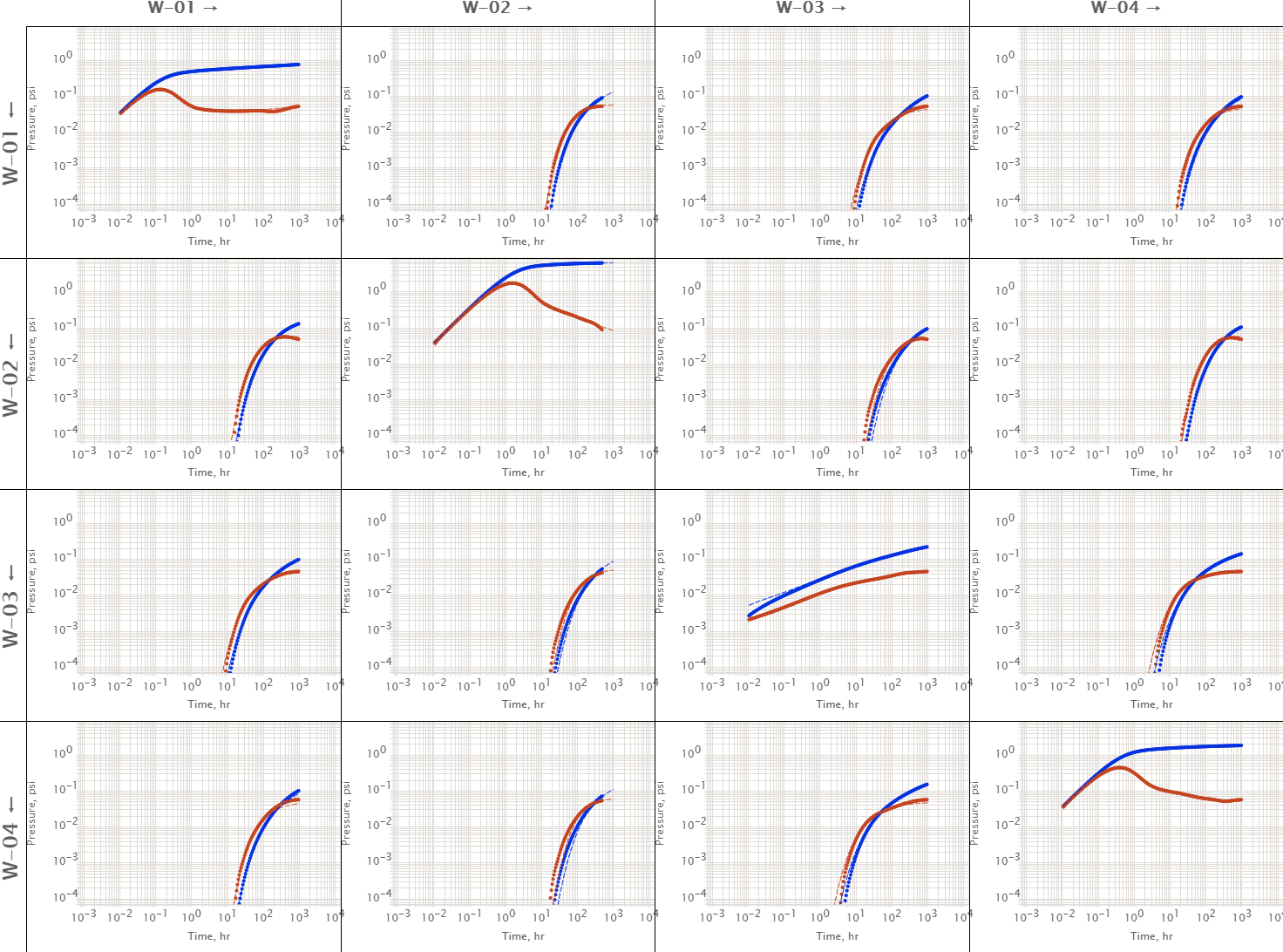 Image Added Image Added
|
Fig. 2. UTR output diagram from XDCV. The column wells showing pressure response to row wells. Diagonal elements are showing self-response DTRs. Non-diagonal elements showing cross-well response CTRs. |
Multiwell deconvolution (MDCV) specifies two types of UTR: Drawdown Transient Response (DTR) and Cross-well Transient Response (CTR).
The Drawdown Transient Response (
| Hint |
|---|
| 0 | DTR |
|---|
| 1 | Drawdown Transient Response |
|---|
| 2 | DTR |
|---|
|
Response (DTR) is the imaginary sandface pressure response of a given well to its its total sandface unit-rate production in absence of the other wellsunder condition that no other well is producing/injecting.It is equivalent to conventional drawdown test Drawdown Test with sandface unit-rate production as if the well is not interfering with surrounding wells.
The Cross-well Transient Response (
| Hint |
|---|
| 0 | CTR |
|---|
| 1 | Cross-well transient response |
|---|
| 2 | CTR |
|---|
|
) is the Response (CTR) is the sandface pressure response of a given well to the the total sandface unit-rate production of the offset well in absence of the other wellswell under condition that no other well is producing/injecting.
It is equivalent to the pressure interference test the Pressure Interference Test with the unit-rate production in disturbing well as if the receiving well is shut-in and no other well .| Hint |
|---|
| 0 | MDCV |
|---|
| 1 | Multiwell deconvolution |
|---|
|
is only working in low-compressibility formations, hence before using | Hint |
|---|
| 0 | MDCV |
|---|
| 1 | Multiwell deconvolution |
|---|
|
one should analyze the data to see if this condition is met for the tested area.is producing/injecting.
Although the UTR may last the infinite time but in reservoir engineering practise the UTR is usually assumed to be captured when it develops a boundary-dominated Late Time Response (LTR). It should be noted that sometimes the duration of production history is too short to sense the geometrical boundary and UTR will not capture it in full or not see a boundary at all.
The true UTRs are also difficult to acquire in practise as most wells are noticeably interferring during at long-term scales. The exception is the remote well or the well draining an isolated compartment.
This defines the application of MDCV which pretends to decipher the UTR from BHP and Production/Injection History.
The pressure convolution principle itself has some limitations and may not be adequate for some practical cases.
For example, changing reservoir conditions, high compressibility – everything which breaks linearity of diffusion equations.
There are some workarounds on these cases but the best practice is to check the validity of pressure convolution (and therefore the applicability of MDCV) on the simple synthetic 2-well Dynamic Flow Model (DFM) with the typical for the given case reservoir-fluid-production conditions.
MDCV
| Hint |
|---|
| 0 | MDCV |
|---|
| 1 | Multiwell deconvolution |
|---|
|
can be performed in two options: Radial Deconvolution (| Hint |
|---|
0 | RDCV| 1 | Radial Deconvolution |
|---|
) and ) and Cross-well Deconvolution (| Hint |
|---|
0 | XDCV| 1 | Cross-well Deconvolution |
|---|
).
Radial Deconvolution Deconvolution (| Hint |
|---|
0 | RDCV| 1 | Radial Deconvolution |
|---|
) corrrelates ) correlates pressure and rate in selected well (called pressure-tested well) and only account for the rates in surrounding wells (called rate-tested wells) in order to reconstruct:- Pressure response of the well to its unit rate production in absence of other wells (also called Diagonal Self-Response or Drawdown Transient Response or
| Hint |
|---|
| 0 | DTR |
|---|
| 1 | Diagonal Transient Response |
|---|
2 | DTR)
- Pressure response of the well to offset well unit rate production in absence of other wells (also called Cross-well Transient Response or
| Hint |
|---|
| 0 | CTR |
|---|
| 1 | Cross-well transient response |
|---|
2 | CTR)
A group of
wells with one selected pressure-tested well has transient responses: 1 diagonal transient response and cross-well transient responses.
The main difference between between RDCV and single-well deconvolution (SDCV ) is that it takes into account offset wells impact on tested well pressure.
Only rates are taken into account for offset wells in RDCV.
In case a group of tested wells have mulitple pressue gauge installations one may wish to deconvolve the unit-rate transient responses using all of the pressure data which is called Cross-well deconvolution (
| Hint |
|---|
| 0 | XDCV |
|---|
| 1 | Cross-well Deconvolution |
|---|
|
Deconvolution (XDCV).
The main advantage of
| Hint |
|---|
| 0 | XDCV |
|---|
| 1 | Cross-well Deconvolution |
|---|
|
over | Hint |
|---|
| 0 | RDCV |
|---|
| 1 | Radial Deconvolution |
|---|
|
XDCV over RDCV is the ability to simulate and interpret all PDG simultaneiouslysimultaneously, resulting in mopre more information and better constrain and stability of deconvolution process.The group of
pressure-tested wells has transient responses, because every well has 1 diagonal transient response and cross-well transient responses thus having transient responses for each well.The intervals between two wells with pressure gauge instaltions installations results in two transient response: first well onto the second well and revers.
This may indicate anisotropy of pressure propagation in counter directions and shed the light on the resevroir physics between these wells.
Once all possible DTR/CTR are deconvolved one can perform a conventional type-curve analysis for each well, defining the type and distance to the boundary, estimating skin, transmissibility and diffusivity around each well.
Unlike routine numericial fitting, where
pressure responses to complicated rate history are being fit for wells, one can run XDCV to get responses to very simple rate history (unit rate production) and then fit them all with diffusion models (sequentially or in parallel) by varying the same parameters (current formation pressure around every well Pe, skin-factor S for every well, and usually, transmissibility σ + pressure diffusivity χ around each well).
Main benefits of | Hint |
|---|
0 | MDCV| 1 | Multiwell deconvolution |
|---|
are:
- Reconstruction of formation pressure history
- Rate corrections for random mistake
- The ability to get transient responses without initial knowledge of reservoir geometry
Main disadvantages of | Hint |
|---|
0 | MDCV| 1 | Multiwell deconvolution |
|---|
are:
- Uncertainty in DTR/CTR, in case of uneventfull production history or synchronized correlated flow variation of two (or more) wells
- Error Uncertainty in DTR/CTR is increasing with the number of wells in the test
Mathematics
In linear formation approхimation the pressure response to the varying rates in the offset wells is subject to convolution equation:
| LaTeX Math Block |
|---|
|
p_n(t) = p_{i,n} + \sum_{k = 1}^N \sum_{\alpha = 1}^{N_k} \big( q^{(\alpha)}_k - q^{(\alpha-1)}_k \big) \ p^u_{nk}(t - t_{\alpha k}) |
where
| 1 | | pressure at -th well at arbitrary moment of time |
| 2 | | initial pressure at -the well |
| 3 | | rate value of -th transient at -th well |
| 4 | | pressure transient response in -th wel to unit-rate production from -th well |
| 5 | | starting point of the -th transient in -th well |
| 6 | | number of wells in the test |
| 7 | | number of transients in -th well |
with assumption:
– for any well at for any pair of wells Hence, convolution is using initial formation pressure
, unit-rate transient responses of wells and cross-well intervals and rate histories | LaTeX Math Inline |
|---|
| body | \{ q_k (t) \}_{k = 1 .. N} |
|---|
|
to calculate pressure bottom-hole pressure response as function time :| LaTeX Math Block |
|---|
|
\big\{ p_{i, n}, \{ p^u_{nk} (t), q_k (t) \}_{k = 1 .. N} \big\} \rightarrow p_n(t) |
The
| Hint |
|---|
| 0 | MDCV |
|---|
| 1 | Multiwell Deconvolution |
|---|
|
is a reverse problem to convolution and search for functions and numbers using the historical pressure and rate records | LaTeX Math Inline |
|---|
| body | \{ p_k(t), \ \{ q^{(\alpha)}_k \}_{\alpha = 1.. N_k} \}_{k = 1 .. N} |
|---|
|
and provides the adjustment to the rate histories for the small mistakes | LaTeX Math Inline |
|---|
| body | \{ q_k \}_{\alpha = 1.. N_k} \rightarrow \{ \tilde q_k \}_{\alpha = 1.. N_k} |
|---|
|
:| LaTeX Math Block |
|---|
|
\big\{ p_k(t), q_k (t) \big\} _{k = 1 .. N} \rightarrow \big\{ p_{i, n}, \{ p^u_{nk} (t), \tilde q_k (t) \}_{k = 1 .. N} \big\} |
The solution of deconvolution problem is based on the minimization of the objective function:
| LaTeX Math Block |
|---|
|
E(\{ p_{i,n}, p^u_{nk}(\tau), q^{(\alpha)}_n \}_{n=1..N}) \rightarrow {\rm min} |
where
| LaTeX Math Block |
|---|
|
E(\{ p_{i,n}, p^u_{nk}(\tau), q^{(\alpha)}_n \}_{n=1..N}) = \sum_{n=1}^N \Big(p_{i,n} + \sum_{k = 1}^N  \sum_{\alpha = 1}^{N_k} (q^{(\alpha)}_k - q^{(\alpha-1)}_k ) \ p^u_{nk}(t - t_{\alpha k})- p_n(t) \Big)^2
+ w_c \, \sum_{n = 1}^N \sum_{k = 1}^{N_k} {\rm Curv} \big( p^u_{nk}(\tau) \big) +
w_q \, \sum_{k = 1}^N \sum_{\alpha = 1}^{N_k} \big( q^{(\alpha)}_k - \tilde q^{(\alpha)}_k \big)^2 |
and objective function components have the following meaning:
| LaTeX Math Inline |
|---|
| body | \sum_{n=1}^N \Big(p_{i,n} + \sum_{k = 1}^N \sum_{\alpha = 1}^{N_k} (q^{(\alpha)}_k - q^{(\alpha-1)}_k ) \ p^u_{nk}(t - t_{\alpha k})- p_n(t) \Big)^2 |
|---|
|
| is responsible for minimizing discrepancy between model and historical pressure data |
| LaTeX Math Inline |
|---|
| body | w_c \, \sum_{n = 1}^N \sum_{k = 1}^{N_k} {\rm Curv} \big( p^u_{nk}(\tau) \big) |
|---|
|
| is responsible for minimizing the curvature of the transient response (which reflects the diffusion character of the pressure response to well flow) |
| LaTeX Math Inline |
|---|
| body | w_q \, \sum_{k = 1}^N \sum_{\alpha = 1}^{N_k} \big( q^{(\alpha)}_k - \tilde q^{(\alpha)}_k \big)^2 |
|---|
|
| is responsible for minimizing discrepancy between model and historical rate data (since historical rate records are not accurate at the time scale of pressure sampling) |
In practice the above approach is not stable.
One of the efficeint regularizations has been suggested by Shroeter
One of the most efficient method in minimizing the above objective function is the hybrid of genetic and quasinewton algorithms in parallel on multicore workstation.
The
| Hint |
|---|
| 0 | MDCV |
|---|
| 1 | Multiwell Deconvolution |
|---|
|
also adjusts the rate histories for each well | LaTeX Math Inline |
|---|
| body | \{ q^{(\alpha)}_k \}_{\alpha = 1.. N_k} \rightarrow \{ \tilde q^{(\alpha)}_k \}_{\alpha = 1.. N_k} |
|---|
|
to achieve the best macth of the bottom hole pressure readings.The weight coefficients
and control contributions from corresponding components and should be calibrated to the reference transients (manuualy or automatically).The
| Hint |
|---|
| 0 | MDCV |
|---|
| 1 | Multiwell Deconvolution |
|---|
|
methodology constitute a big area of practical knowledge and not all the tricks and solutions are currenlty automated and require a practical skill. Sample
Sample #1 – RDCV
На рис. 2.1.2 представлена карта участка с тремя скважинами.
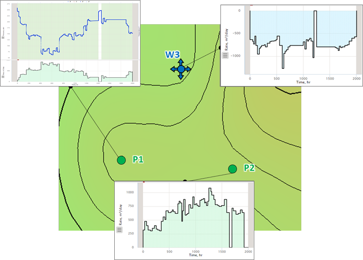 Image Removed
Синтетическая история работы добывающей скважины с простым поведением продуктивности.
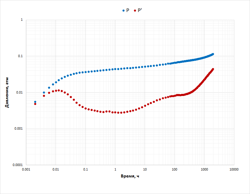 Image Removed Image Removed
|
| Рис. 2.1.2. Скв. Р1. Мультискважинная деконволюция |
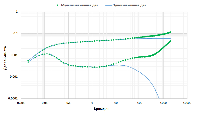 Image Removed Image Removed
|
Рис. 2.1.3. Скв. Р1.Сравнение мультискважинной деконволюции с односкважинной деконволюциейНа Рис. 2.1.4 приведена история дебитов и давлений по всем скважинам. Image Removed Image Removed
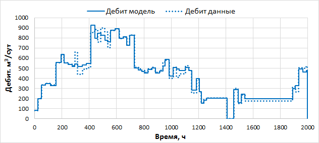 Image Removed Image Removed
|
Рис. 2.1.4. P1. Сравнение полученной истории дебитов и давления с исходными |
Пример #2 – КДКВ
На Рис. 2.1.5 представлена карта участка с тремя скважинами.
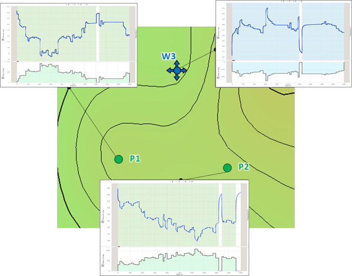 Image Removed Image Removed
|
Рис. 2.1.5. Синтетическая история работы добывающей скважины с простым поведением продуктивности |
Image Removed |
| Рис. 2.1.6. Скв. Р1. Сравнение мультискважинной деконволюции и односкважинной деконволюции |
 Image Removed Image Removed
|
Рис. 2.1.7. Влияние скважины P2 на скважину P1 |
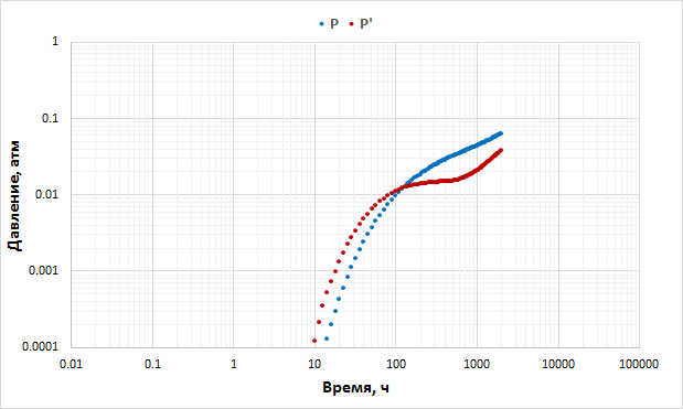 Image Removed
| Рис. 2.1.8. Влияние скважины W3 на скважину P1 |
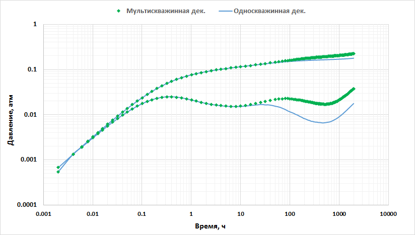 Image Removed Image Removed
|
Рис. 2.1.9. Скв. Р2. Сравнение мультискважинной деконволюции и односкважинной деконволюции |
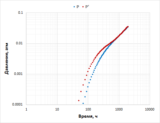 Image Removed
| Рис. 2.1.10. Влияние скважины 1 на скважину 2 |
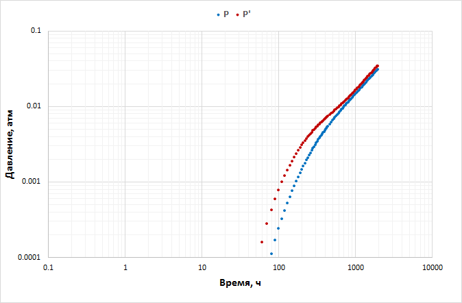 Image Removed Image Removed
|
| Рис. 2.1.11. Влияние скважины W3 на скважину P2 |
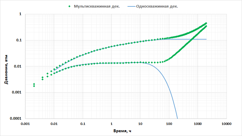 Image Removed Image Removed
|
| Рис. 2.1.12. Сравнение мультискважинной деконволюции и односкважинной деконволюции |
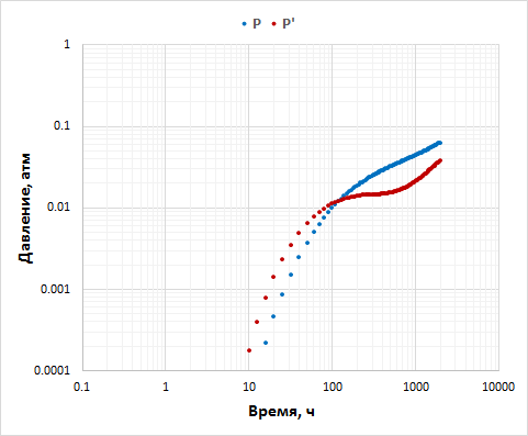 Image Removed Image Removed
|
| Рис. 2.1.13. Влияние скважины P1 на скважину W3 |
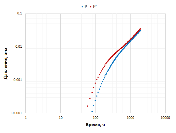 Image Removed Image Removed
|
| Рис. 2.1.14. Скв. W3 Влияние скважины P2 на скважину W3 |
На Рис. 2.1.15 приведена история дебитов и давлений по всем скважинам.
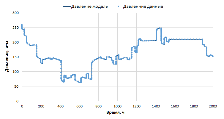 Image Removed Image Removed
 Image Removed Image Removed
|
Рис. 2.1.15. P1. Сравнение полученной истории дебитов и давления с исходными |
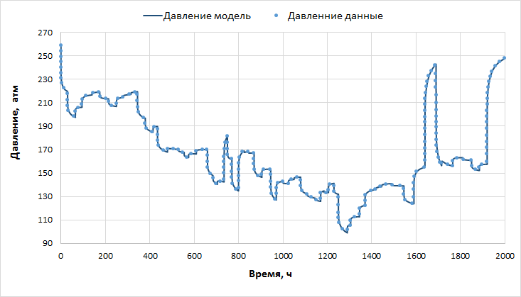 Image Removed Image Removed
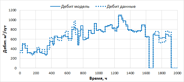 Image Removed Image Removed
|
| Рис. 2.1.16. P2. Сравнение полученной истории дебитов и давления с исходными |
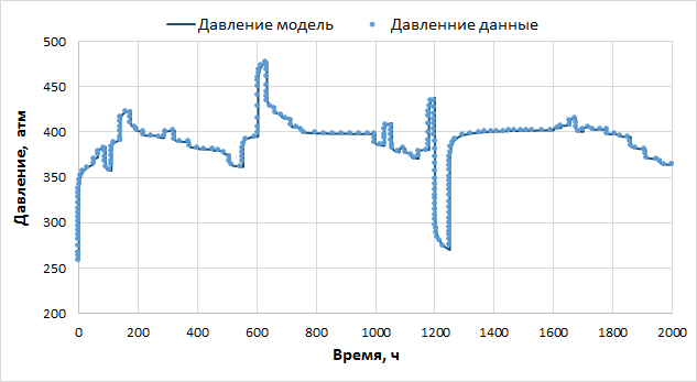 Image Removed Image Removed
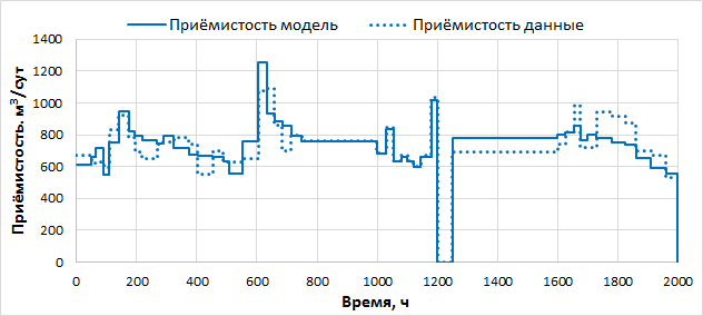 Image Removed Image Removed
|
Рис. 2.1.17. W3. Сравнение полученной истории дебитов и давления с исходными
...