...

Expand

title	PRIME Mathematics

Property Abbrevy

Property Name

Formula

VRR_cum

Cumulative Voidage Replacement Ratio

LaTeX Math Block

anchor	1
alignment	left

{\rm VRR_{cum}} = \frac{B_w \, Q_{WI}}{B_w \, Q_W + B_o \, Q_O + B_g Q_G - B_g R_s Q_O}

VRRcur

Current Voidage Replacement Ratio

(month over month)

LaTeX Math Block

anchor	1
alignment	left

{\rm VRR_{cur}} = \frac{B_w \, q_{WI}}{B_w \, q_W + B_o \, q_O + B_g (q_G - R_s Q_O)}

RF

Recovery Factor

LaTeX Math Block

anchor	1
alignment	left

{\rm RF} = \frac{Q_O}{V_{STOIIP}}

Y_w

Watercut (production)

LaTeX Math Block

anchor	1
alignment	left

{\rm Y_w} = \frac{q_W}{q_{LIQ}}

Y_wm

Watercut (proxy-model)

LaTeX Math Block

anchor	1
alignment	left

{\rm Y_{wm}} = \frac{1}{1 + \frac{K_{ro}}{K_{rw}} \cdot \frac{ \mu_w}{\mu_o}  \cdot \frac{B_w}{B_o} }

LaTeX Math Block

anchor	1
alignment	left

s_w = \frac{Q_o \, B_o}{V_\phi}

GOR

Gas-Oil Ratio (production)

LaTeX Math Block

anchor	1
alignment	left

{\rm GOR} = \frac{q_g}{q_o}

GOR_m

Gas-Oil Ratio (proxy-model)

LaTeX Math Block

anchor	1
alignment	left

{\rm GOR_m} = R_s +  \frac{k_{rg}}{k_{ro}} 
\cdot \frac{\mu_o}{\mu_g} 
\cdot \frac{B_o }{B_g}

q_LIQ

Liquid rate

LaTeX Math Block

anchor	1
alignment	left

q_{LIQ} = q_O + q_W

PIR

Production Injection Ratio (production)

LaTeX Math Block

anchor	1
alignment	left

{\rm PIR} = \frac{Q_O}{Q_{WI}}

PIR_m

Production Injection Ratio (model)

LaTeX Math Block

anchor	1
alignment	left

{\rm PIR_m} = { \frac{1}{VRR} } \cdot { \frac{1-Y_w}{ Y_w + (1-Y_w) \bigg[ \frac{B_o}{B_w} - \frac{B_g}{B_w}(GOR - R_s) \bigg] } }

J_O

Oil Productivity Index

LaTeX Math Block

anchor	1
alignment	left

{\rm J_{O}} = \frac{q_O}{P_e - P_{wf}} {\quad \Rightarrow \quad} P_{wf} = P_e - \frac{1}{J_O} q_O

J_PI

Total Productivity Index (production)

LaTeX Math Block

anchor	1
alignment	left

{\rm J_t} = \frac{q_t}{P_e - P_{wf}}

J_PIm

Total Productivity Index (model)

LaTeX Math Block

anchor	1
alignment	left

{\rm J_{tm} } = \frac{2 \pi \sigma}{\ln \frac{r_e}{r_w} +0.5 + S}

_jPI

Total Specific Productivity Index

LaTeX Math Block

anchor	1
alignment	left

{\rm j_t} = \frac{q_t}{h \cdot (P_e - P_{wf})}

_jPIm

Total Specific Productivity Index (model)

LaTeX Math Block

anchor	1
alignment	left

{\rm j_{tm} } = \frac{2 \pi <k/\mu>}{\ln \frac{r_e}{r_w} +0.5 + S}

Expand

title	Derivation of PIR equation

LaTeX Math Block

anchor	1
alignment	left

VRR = \frac{B_w \, q_{WI}}{B_w \, q_W + B_o \, q_O + B_g \, [ q_G - R_s \, q_O] } =  \frac{B_w \, q_{WI}}{B_w \, q_W + B_o \, q_O + B_g \, [ GOR - R_s] q_O } = \frac{B_w \, q_{WI}}{B_w \, q_W + [ B_o  + B_g \, ( GOR - R_s) ] \, q_O }

LaTeX Math Block

anchor	1
alignment	left

VRR = \frac{q_{WI}}{q_W + \bigg[ \frac{B_o}{B_w}  + \frac{B_g}{B_w} \, ( GOR - R_s) \bigg] \, q_O }

LaTeX Math Block

anchor	1
alignment	left

Y_w=\frac{q_W}{q_W + q_O} \rightarrow \frac{q_O}{q_W} = \frac{1-Y_w}{Y_w} \rightarrow q_W =  \frac{Y_w}{1-Y_w} \, q_O

LaTeX Math Block

anchor	1
alignment	left

VRR =  \frac{q_{WI}}{q_O} \cdot \frac{1}{\frac{Y_w}{1-Y_w}  + \bigg[ \frac{B_o}{B_w}  + \frac{B_g}{B_w} \, ( GOR - R_s) \bigg] } =
\frac{q_{WI}}{q_O} \cdot \frac{1-Y_w}{Y_w  + (1-Y_w) \, \bigg[ \frac{B_o}{B_w}  + \frac{B_g}{B_w} \, ( GOR - R_s) \bigg] }

LaTeX Math Block

anchor	1
alignment	left

PIR=\frac{q_W}{q_{WI}} = \frac{1}{VRR} \cdot \frac{1-Y_w}{Y_w  + (1-Y_w) \, \bigg[ \frac{B_o}{B_w}  + \frac{B_g}{B_w} \, ( GOR - R_s) \bigg] }

› PRIME Diagnostics

Sample Case 1 – Waterflood Sector Analysis

...


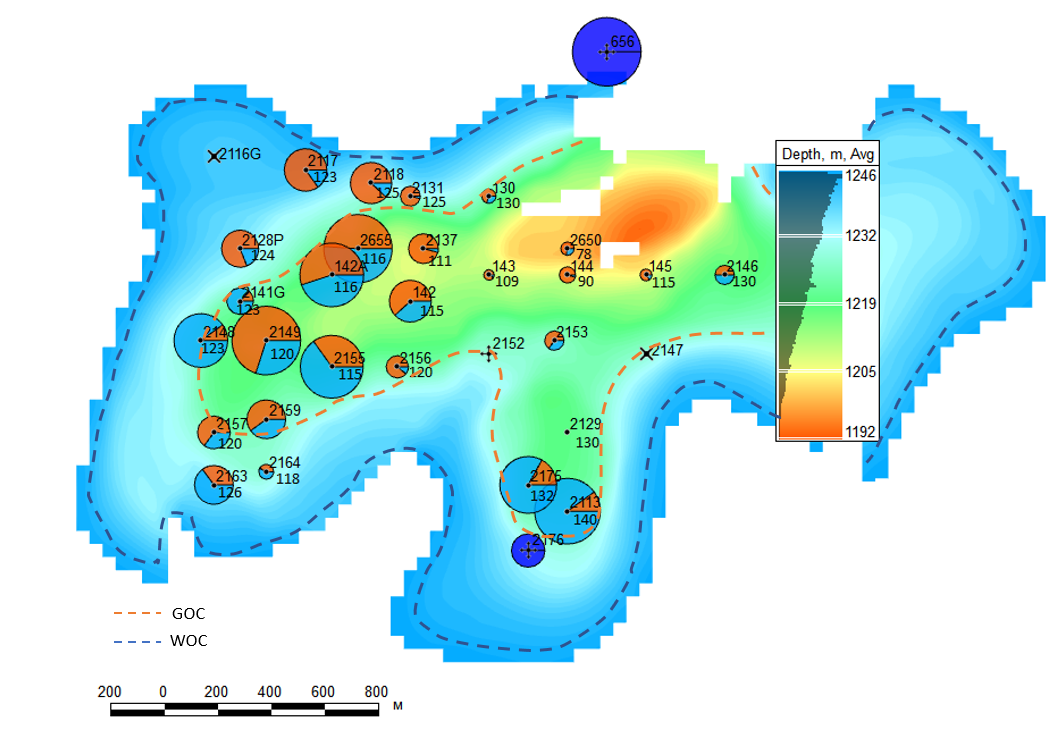
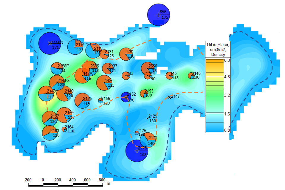
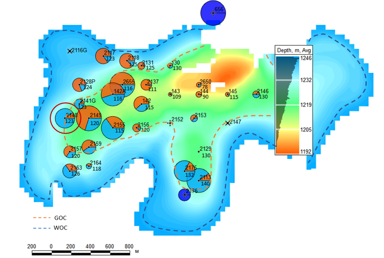
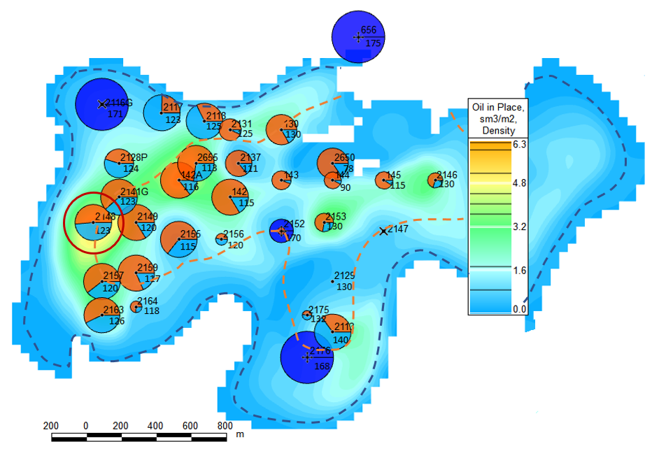
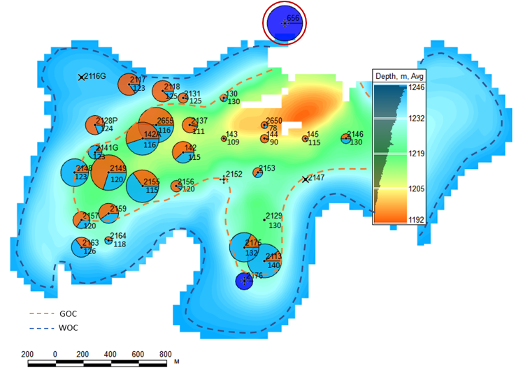
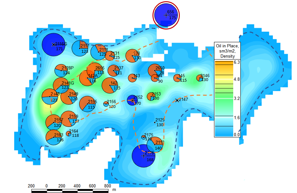
Fig. 1.1. Production History Map	Fig. 1.2. Recovery Map


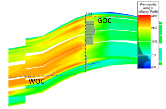
Fig. 2.1. Cross-section & PLT, permeability, GOC, OWC	Fig. 2.2. Cross-section & PLT, permeability, GOC, OWC


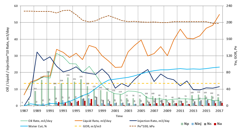
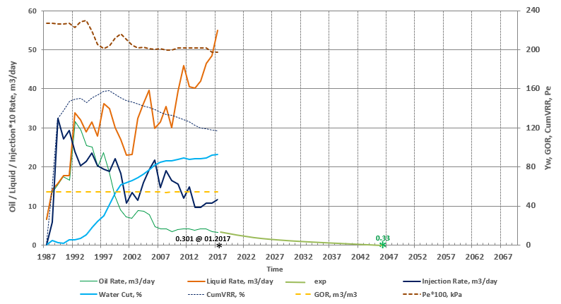
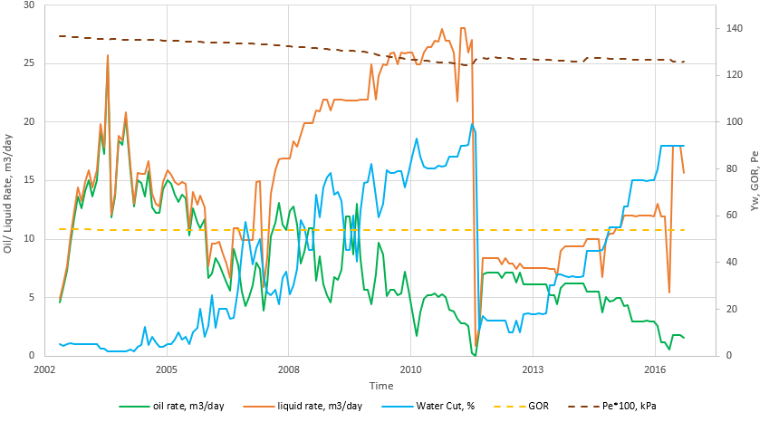
Fig. 3.1. Production History Graphs	Fig. 3.2. Production Forecasts


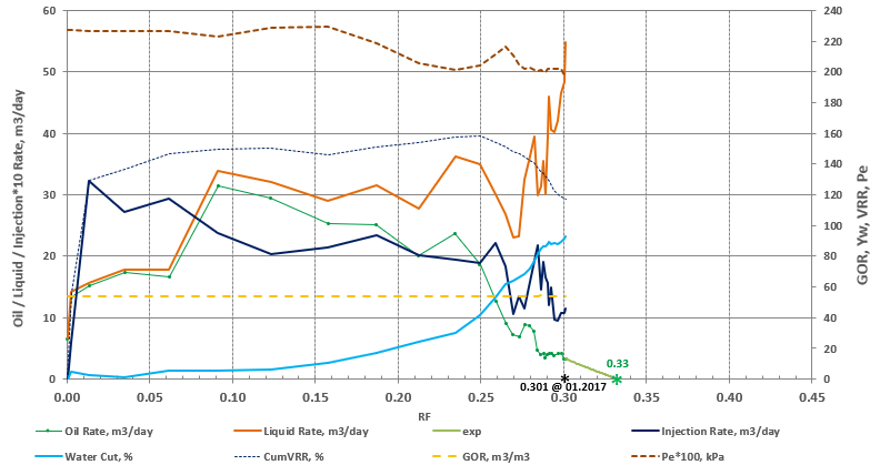
Fig. 4.1. Recovery History	Fig. 4.2. Recovery Forecasts


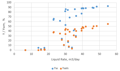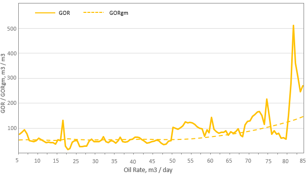Fig. 5.1. WOR Diagnostic	Fig. 5.2.. GOR Diagnostic


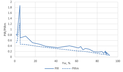
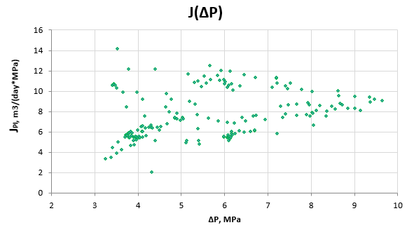
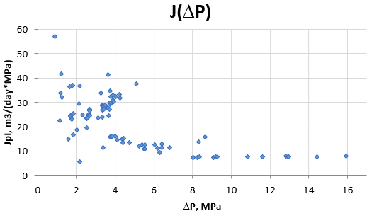
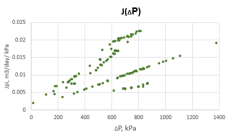
Fig. 6. 71. Productivity Index Diagnostic	Fig. 6. 72. Injectivity Index Diagnostic


Fig. 67. Injection Efficiency Diagnostics

Sample Case 2 – Oil Producer Analysis

...


Fig. 1. Production History Map	Fig. 2. Recovery Map	Fig. 3. Cross-section & PLT


Fig. 4. Production History Graphs	Fig. 5. Decline Curve Analysis	Fig. 6. Recovery Diagnostic


Fig. 7. Watercut Diagnostic	Fig. 8. GOR Diagnostic	Fig. 9. Injection Efficiency Diagnostics


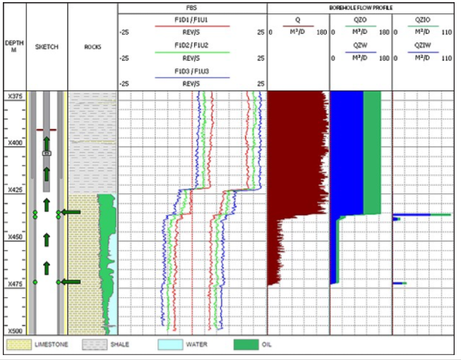
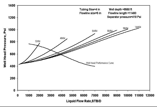
Fig. 10. Well Performance Analysis (VFP + IPR)	Fig. 11. Productivity Index Diagnostic	Fig. 12. Well Completion & PLT

Sample Case 3 – Water Injector Analysis

...


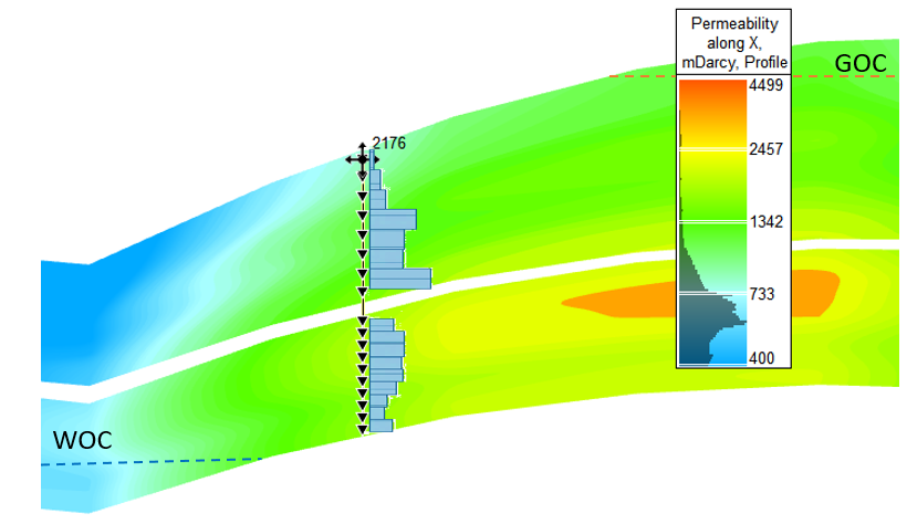Fig. 1. Production History Map	Fig. 2. Recovery Map	Fig. 3. Cross-section & PLT


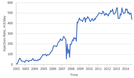
Fig. 4. Injection History Graphs


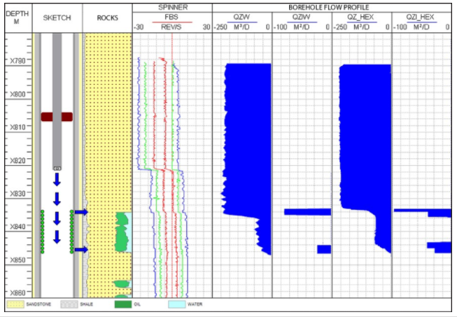
Fig. 10. Well Performance Analysis (VFP + IPR)	Fig. 11. Injectivity Index Diagnostic	Fig. 12. Well Completion & PLT