Specific Production Analysis workflow with basic Production Performance Metrics.
| Application | Sample Cases |
|---|---|
| First guess on redevelopment opportunities | Natural Depletion Reservoir |
| Identify and prioritise surveillance opportunities | Waterflood Sector Analysis |
| Assess current production performance: | Oil Producer Analysis |
|
Definition
Primary Production Analysis is the specific workflow and report template on Primary Well & Reservoir Performance Indicators.
Application
...
|
...
...
|
...
|
...
|
...
Technology
Primary Production Analysis is built around production data against material balance and require current FDP volumetrics, PVT and SCAL models.
It includes well-by-well diagnostics and gross field diagnostics, but may be extended to sector-by-sector diagnostics.
Metrics
Primary Production Analysis includes the following metrics:
...
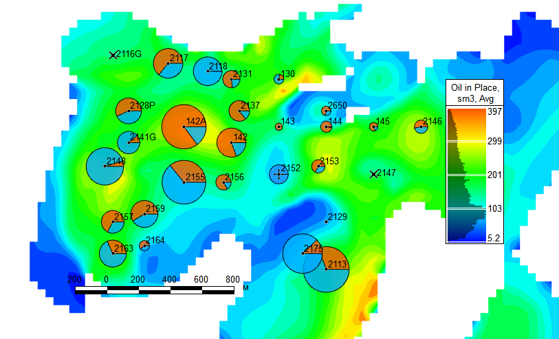
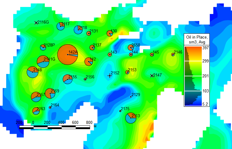
Background = STOIIP & Structure
Bubbles = qo, qg , qw, qinj
Number = CurVRR, Pe
...
Background = STOIIP & Structure
Bubbles = Qo, Qg , Qw, Qinj
Number = CumVRR, Pe
...
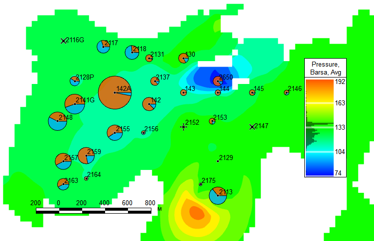
Background = STOIIP & Structure
Bubbles = VRR
Number = Pe / Pem
...
Left Axis = qo, qg , qw, qinj,
Rigth Axis = Yw, GOR, Pe , Np, Ninj
Hor Axis = Elapsed Time
...
Decline Curve Analysis
...
Left Axis = qo1, qliq1, qinj1,
Rigth Axis = Yw, GOR, VRR, Pe
Hor Axis = Elapsed Time
...
Left Axis = qo1, qliq1, qinj1
Rigth Axis =Yw, GOR, VRR, Pe, Pem
Hor Axis = RF
...
Left Axis = Yw, Ywm
Hor Axis = qliq
...
Left Axis = GOR, GORgm
Hor Axis =qo
...
Injection Efficiency Diagnostics
...
Left Axis = PIR , PIRm
Hor Axis = Yw
...
Left Axis = Pwf_IPR , Pwf_VLP
Hor Axis = qo
...
Productivity Index Diagnostic
...
Left Axis = JPI, JPIm
Hor Axis = dP = Pwf - Pe
...
Below is the list of the production properties involved on the above metrics.
...
Cumulative Voidage Replacement Ratio
...
| LaTeX Math Block | ||||
|---|---|---|---|---|
| ||||
{\rm VRR_{cum}} = \frac{B_w \, Q_{WI}}{B_w \, Q_W + B_o \, Q_O + B_g Q_G - B_g R_s Q_O} |
...
| LaTeX Math Block | ||||
|---|---|---|---|---|
| ||||
{\rm VRR_{inst}} = \frac{B_w \, q_{WI}}{B_w \, q_W + B_o \, q_O + B_g (q_G - R_s Q_O)} |
...
Recovery Factor
...
| LaTeX Math Block | ||||
|---|---|---|---|---|
| ||||
{\rm RF} = \frac{Q_O}{V_{STOIIP}} |
...
Watercut
| LaTeX Math Block | ||||
|---|---|---|---|---|
| ||||
{\rm Y_w} = \frac{q_W}{q_{LIQ}} |
...
| LaTeX Math Block | ||||
|---|---|---|---|---|
| ||||
{\rm Y_{wm}} = \frac{1}{1 + \frac{K_{ro}}{K_{rw}} \cdot \frac{\mu_w}{\mu_o} \cdot \frac{B_w}{B_o}} |
...
| LaTeX Math Block | ||||
|---|---|---|---|---|
| ||||
{\rm GOR} = \frac{q_g}{q_o} |
...
| LaTeX Math Block | ||||
|---|---|---|---|---|
| ||||
{\rm GOR_m} = R_s + \frac{B_o \, \mu_o}{B_g \, \mu_g} \cdot \frac{k_{rg}}{k_{ro}} |
...
| LaTeX Math Block | ||||
|---|---|---|---|---|
| ||||
q_{LIQ} = q_O + q_W |
...
PIR
Production Injection Ratio
| LaTeX Math Block | ||||
|---|---|---|---|---|
| ||||
{\rm PIR} = \frac{Q_O}{Q_{WI}} |
...
| LaTeX Math Block | ||||
|---|---|---|---|---|
| ||||
{\rm PIR_m} = { \frac{1}{VRR} } \cdot { \frac{1-Y_w}{ Y_w + (1-Y_w) \bigg[ \frac{B_o}{B_w} - \frac{B_g}{B_w}(GOR - R_s) \bigg] } } |
...
| LaTeX Math Block | ||||
|---|---|---|---|---|
| ||||
{\rm J_{O}} = \frac{q_O}{P_e - P_{wf}} {\quad \Rightarrow \quad} P_{wf} = P_e - \frac{1}{J_O} q_O |
...
JPI
Total Productivity Index
| LaTeX Math Block | ||||
|---|---|---|---|---|
| ||||
{\rm J_t} = \frac{q_t}{P_e - P_{wf}} |
...
| LaTeX Math Block | ||||
|---|---|---|---|---|
| ||||
{\rm J_{tm} } = \frac{2 \pi \sigma}{\ln \frac{r_e}{r_w} +0.5 + S} |
...
| title | PIR equation deduction |
|---|
| LaTeX Math Block | ||||
|---|---|---|---|---|
| ||||
VRR = \frac{B_w \, q_{WI}}{B_w \, q_W + B_o \, q_O + B_g \, [ q_G - R_s \, q_O] } = \frac{B_w \, q_{WI}}{B_w \, q_W + B_o \, q_O + B_g \, [ GOR - R_s] q_O } = \frac{B_w \, q_{WI}}{B_w \, q_W + [ B_o + B_g \, ( GOR - R_s) ] \, q_O } |
| LaTeX Math Block | ||||
|---|---|---|---|---|
| ||||
VRR = \frac{q_{WI}}{q_W + \bigg[ \frac{B_o}{B_w} + \frac{B_g}{B_w} \, ( GOR - R_s) \bigg] \, q_O } |
| LaTeX Math Block | ||||
|---|---|---|---|---|
| ||||
Y_w=\frac{q_W}{q_W + q_O} \rightarrow \frac{q_O}{q_W} = \frac{1-Y_w}{Y_w} \rightarrow q_W = \frac{Y_w}{1-Y_w} \, q_O |
| LaTeX Math Block | ||||
|---|---|---|---|---|
| ||||
VRR =  \frac{q_{WI}}{q_O} \cdot \frac{1}{\frac{Y_w}{1-Y_w}  + \bigg[ \frac{B_o}{B_w}  + \frac{B_g}{B_w} \, ( GOR - R_s) \bigg] } =
\frac{q_{WI}}{q_O} \cdot \frac{1-Y_w}{Y_w + (1-Y_w) \, \bigg[ \frac{B_o}{B_w} + \frac{B_g}{B_w} \, ( GOR - R_s) \bigg] } |
| LaTeX Math Block | ||||
|---|---|---|---|---|
| ||||
PIR=\frac{q_W}{q_{WI}} = \frac{1}{VRR} \cdot \frac{1-Y_w}{Y_w + (1-Y_w) \, \bigg[ \frac{B_o}{B_w} + \frac{B_g}{B_w} \, ( GOR - R_s) \bigg] } |
Diagnostic
...
| title | Expand |
|---|
...
| group | sofoil |
|---|
Введение
История добычи
...
Карты разработки
...
Падающая добыча
Стационарная добыча
Стационарная добыча это режим в котором давление на линии отбора поддерживается постоянным за счет газовой шапки, аквифера или закачки в нагнетательные скважины.
Растущая добыча
Динамика пластового давления
...
| |
|
| Advantages | Limitations |
|---|---|
| Fast Track | Short production forecasts only |
| Minimal input data | Sometimes incapable to forecast |
| Straightforward analysis | High level hint of reserves distribution only |
| Fair hints for underperforming wells and sectors |
See Also
...
Petroleum Industry / Upstream / Production / Subsurface Production / Field Study & Modelling / Production Analysis
[ Production Performance Indicators @model ]
[ Dynamic Data Statistical Correlation ]
[ Well Location and Flow Rate Map ]
Снижение пластового давления приводит к снижению пористости и проницаемости коллектора, что приводит к потере продуктивности и снижению дебита сквжаины.
Снижение пластового давления ниже давления насыщения приводит к выделению газа в призабойной зоне и потере продуктивности скважин по жидкости за счет более высокой мобильности газа и за счет дроссельного охлаждения, что в итоге приводит к снижению дебита скважины.
Диагностические графики анализа добычи NDR
q1o vs RF
...
| LaTeX Math Block | ||||
|---|---|---|---|---|
| ||||
q_{1o} = \frac{\sum Q_o }{ \sum {t_o}} |
| LaTeX Math Block | ||||
|---|---|---|---|---|
| ||||
RF = \frac{\sum_t Q_o }{V_{STOIIP}} |
Yw vs RF
Рис. 1. График обводненности от КИН
Pe vs RF
Диагностические графики анализа заводнения WIR
Sample Case
...
...
...
...
Fig. 1. Production History Map
...
...
...

...