Specific Production Analysis workflow with basic Production Performance Metrics.
| Application | Sample Cases |
|---|---|
| First guess on redevelopment opportunities | Natural Depletion Reservoir |
| Identify and prioritise surveillance opportunities | Waterflood Sector Analysis |
...
| title | Content |
|---|
| Column | |||||||||||||
|---|---|---|---|---|---|---|---|---|---|---|---|---|---|
| |||||||||||||
|
...
| width | 30% |
|---|
Definition
Primary Production Analysis is the specific workflow and report template on Primary Well & Reservoir Performance Indicators.
...
| Assess current production performance |
...
...
|
...
|
...
| Water Injector Analysis |
|
...
|
...
|
...
Limitations
...
Technology
Primary Production Analysis is built around production data against material balance and require current FDP volumetrics, PVT and SCAL models.
The PRIME workflow has certain specifics for oil producers, water injectors, gas injectors and field/sector analysis.
...
| title | PRIME Metrics |
|---|
...
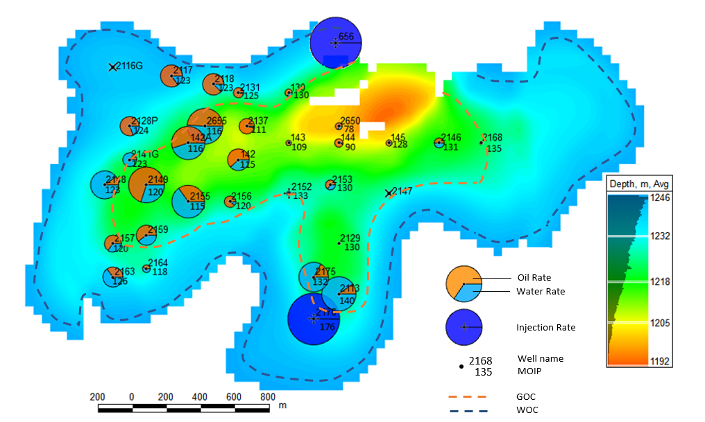
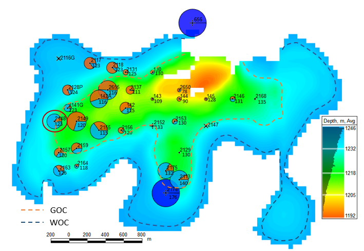
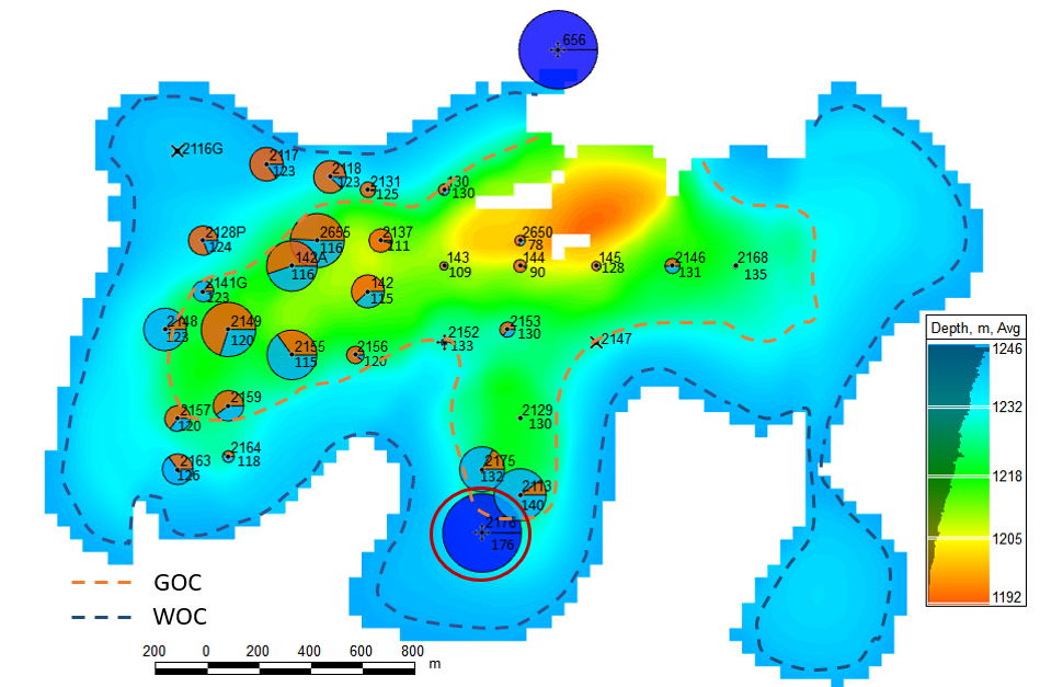
Background = Structure
Bubbles = qo, qg , qw, qinj
Number = CurVRR, Pe
...
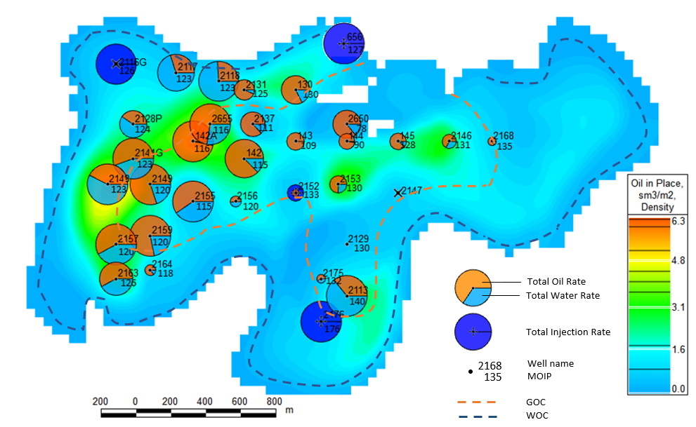
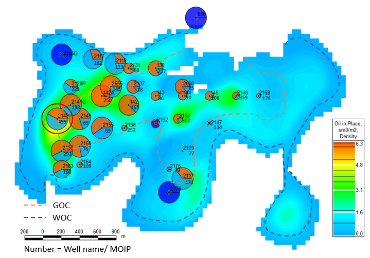
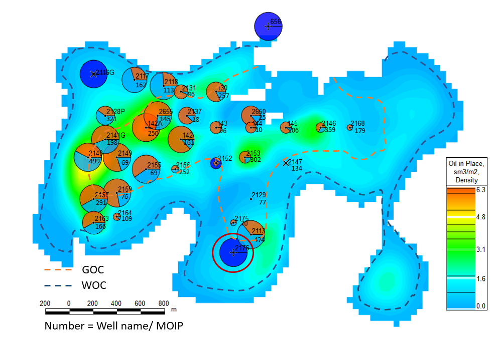
Background = STOIIP
Bubbles = Qo, Qg , Qw, Qinj
Number = CumVRR, Pe
...
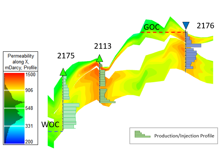
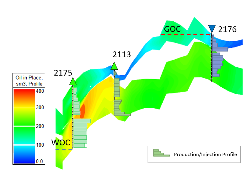
Background = STOIIP & Structure
Bubbles = VRR
Number = Pe , Pem
...
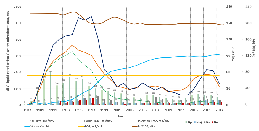
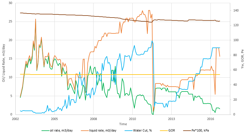
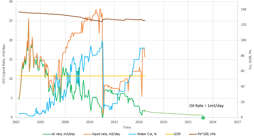
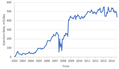
Left Axis = qo, qg , qw, qinj,
Rigth Axis = Yw, GOR, Pe , Np, Ninj
Hor Axis = Elapsed Time
...
Decline Curve Analysis
...
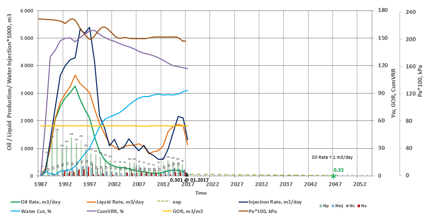
Left Axis = qo1, qliq1, qinj1,
Rigth Axis = Yw, GOR, VRR, Pe
Hor Axis = Elapsed Time
...
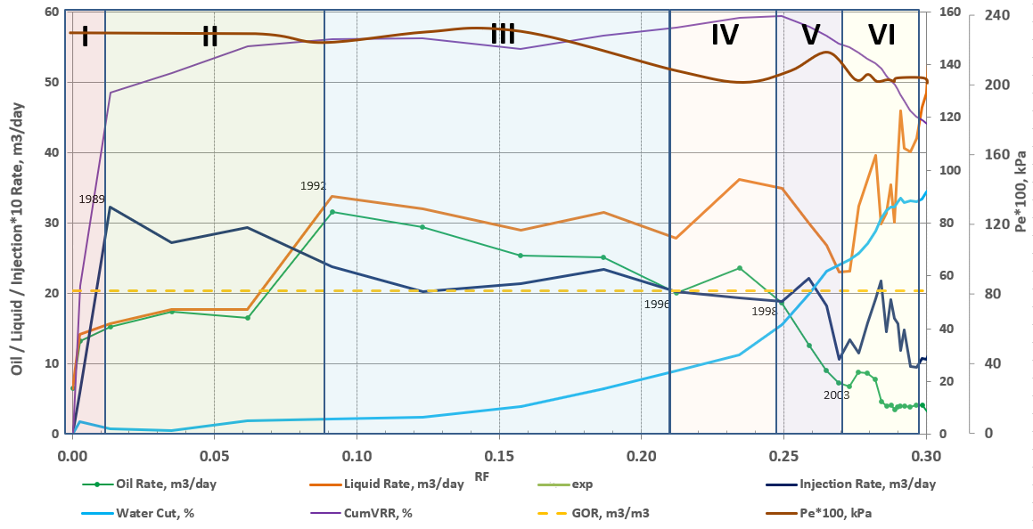
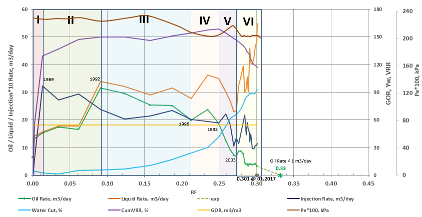
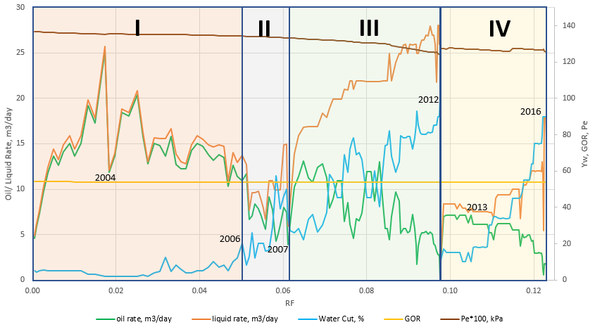
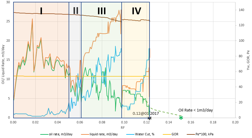
Left Axis = qo1, qliq1, qinj1
Rigth Axis =Yw, GOR, VRR, Pe, Pem
Hor Axis = RF
...
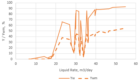
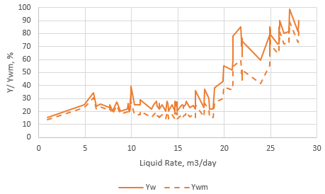
Left Axis = Yw, Ywm
Hor Axis = qliq
...
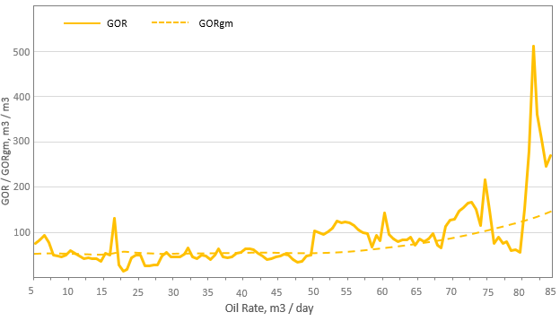
Left Axis = GOR, GORgm
Hor Axis =qo
...
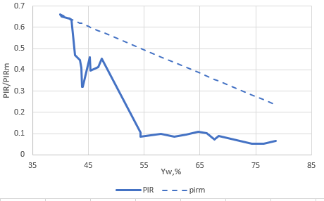
Injection Efficiency Diagnostics
...
Left Axis = PIR , PIRm
Hor Axis = Yw
...
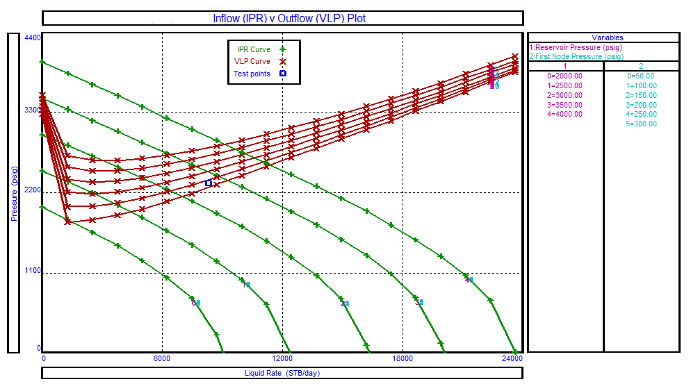
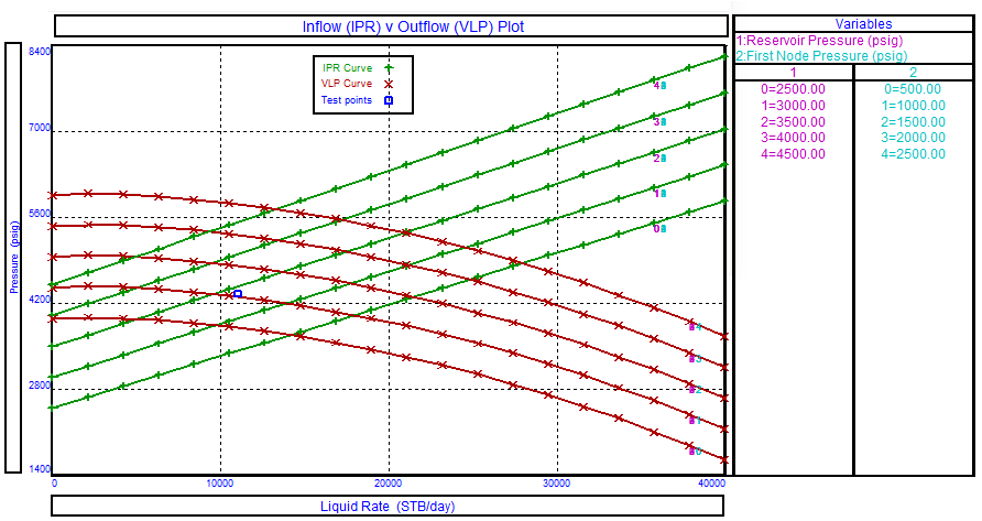
Left Axis = Pwf_IPR , Pwf_VLP
Hor Axis = qo
...
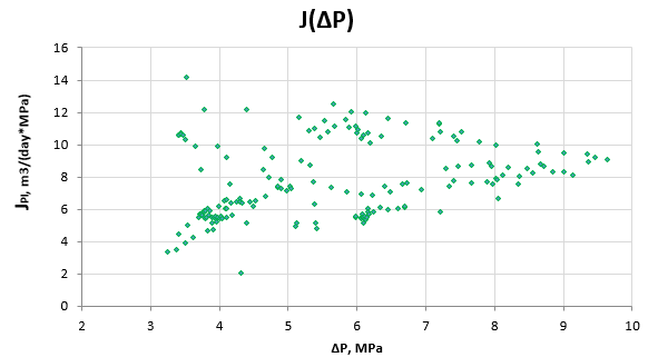
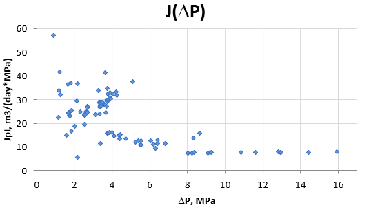
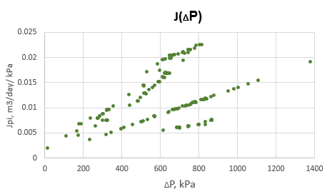
Productivity Index Diagnostic
...
Left Axis = JPI, JPIm
Hor Axis = dP = Pwf - Pe
...
| title | PRIME Mathematics |
|---|
...
Cumulative Voidage Replacement Ratio
...
| LaTeX Math Block | ||||
|---|---|---|---|---|
| ||||
{\rm VRR_{cum}} = \frac{B_w \, Q_{WI}}{B_w \, Q_W + B_o \, Q_O + B_g Q_G - B_g R_s Q_O} |
...
Current Voidage Replacement Ratio
(month over month)
...
| LaTeX Math Block | ||||
|---|---|---|---|---|
| ||||
{\rm VRR_{cur}} = \frac{B_w \, q_{WI}}{B_w \, q_W + B_o \, q_O + B_g (q_G - R_s Q_O)} |
...
Recovery Factor
...
| LaTeX Math Block | ||||
|---|---|---|---|---|
| ||||
{\rm RF} = \frac{Q_O}{V_{STOIIP}} |
...
Watercut (production)
| LaTeX Math Block | ||||
|---|---|---|---|---|
| ||||
{\rm Y_w} = \frac{q_W}{q_{LIQ}} |
...
| LaTeX Math Block | ||||
|---|---|---|---|---|
| ||||
{\rm Y_{wm}} = \frac{1}{1 + \frac{K_{ro}}{K_{rw}} \cdot \frac{ \mu_w}{\mu_o} \cdot \frac{B_w}{B_o} } |
| LaTeX Math Block | ||||
|---|---|---|---|---|
| ||||
s_w = \frac{Q_o \, B_o}{V_\phi} |
...
| LaTeX Math Block | ||||
|---|---|---|---|---|
| ||||
{\rm GOR} = \frac{q_g}{q_o} |
...
| LaTeX Math Block | ||||
|---|---|---|---|---|
| ||||
{\rm GOR_m} = R_s +  \frac{k_{rg}}{k_{ro}}
\cdot \frac{\mu_o}{\mu_g}
\cdot \frac{B_o }{B_g} |
...
| LaTeX Math Block | ||||
|---|---|---|---|---|
| ||||
q_{LIQ} = q_O + q_W |
...
PIR
Production Injection Ratio (production)
| LaTeX Math Block | ||||
|---|---|---|---|---|
| ||||
{\rm PIR} = \frac{Q_O}{Q_{WI}} |
...
| LaTeX Math Block | ||||
|---|---|---|---|---|
| ||||
{\rm PIR_m} = { \frac{1}{VRR} } \cdot { \frac{1-Y_w}{ Y_w + (1-Y_w) \bigg[ \frac{B_o}{B_w} - \frac{B_g}{B_w}(GOR - R_s) \bigg] } } |
...
| LaTeX Math Block | ||||
|---|---|---|---|---|
| ||||
{\rm J_{O}} = \frac{q_O}{P_e - P_{wf}} {\quad \Rightarrow \quad} P_{wf} = P_e - \frac{1}{J_O} q_O |
...
JPI
Total Productivity Index (production)
| LaTeX Math Block | ||||
|---|---|---|---|---|
| ||||
{\rm J_t} = \frac{q_t}{P_e - P_{wf}} |
...
| LaTeX Math Block | ||||
|---|---|---|---|---|
| ||||
{\rm J_{tm} } = \frac{2 \pi \sigma}{\ln \frac{r_e}{r_w} +0.5 + S} |
...
| LaTeX Math Block | ||||
|---|---|---|---|---|
| ||||
{\rm j_t} = \frac{q_t}{h \cdot (P_e - P_{wf})} |
...
| LaTeX Math Block | ||||
|---|---|---|---|---|
| ||||
{\rm j_{tm} } = \frac{2 \pi <k/\mu>}{\ln \frac{r_e}{r_w} +0.5 + S} |
...
| title | Derivation of PIR equation |
|---|
| LaTeX Math Block | ||||
|---|---|---|---|---|
| ||||
VRR = \frac{B_w \, q_{WI}}{B_w \, q_W + B_o \, q_O + B_g \, [ q_G - R_s \, q_O] } = \frac{B_w \, q_{WI}}{B_w \, q_W + B_o \, q_O + B_g \, [ GOR - R_s] q_O } = \frac{B_w \, q_{WI}}{B_w \, q_W + [ B_o + B_g \, ( GOR - R_s) ] \, q_O } |
| LaTeX Math Block | ||||
|---|---|---|---|---|
| ||||
VRR = \frac{q_{WI}}{q_W + \bigg[ \frac{B_o}{B_w} + \frac{B_g}{B_w} \, ( GOR - R_s) \bigg] \, q_O } |
| LaTeX Math Block | ||||
|---|---|---|---|---|
| ||||
Y_w=\frac{q_W}{q_W + q_O} \rightarrow \frac{q_O}{q_W} = \frac{1-Y_w}{Y_w} \rightarrow q_W = \frac{Y_w}{1-Y_w} \, q_O |
| |
|
| Advantages | Limitations |
|---|---|
| Fast Track | Short production forecasts only |
| Minimal input data | Sometimes incapable to forecast |
| Straightforward analysis | High level hint of reserves distribution only |
| Fair hints for underperforming wells and sectors |
See Also
...
Petroleum Industry / Upstream / Production / Subsurface Production / Field Study & Modelling / Production Analysis
[ Production Performance Indicators @model ]
[ Dynamic Data Statistical Correlation ]
[ Well Location and Flow Rate Map ]
| LaTeX Math Block | ||||
|---|---|---|---|---|
| ||||
VRR =  \frac{q_{WI}}{q_O} \cdot \frac{1}{\frac{Y_w}{1-Y_w}  + \bigg[ \frac{B_o}{B_w}  + \frac{B_g}{B_w} \, ( GOR - R_s) \bigg] } =
\frac{q_{WI}}{q_O} \cdot \frac{1-Y_w}{Y_w + (1-Y_w) \, \bigg[ \frac{B_o}{B_w} + \frac{B_g}{B_w} \, ( GOR - R_s) \bigg] } |
| LaTeX Math Block | ||||
|---|---|---|---|---|
| ||||
PIR=\frac{q_O}{q_{WI}} = \frac{1}{VRR} \cdot \frac{1-Y_w}{Y_w + (1-Y_w) \, \bigg[ \frac{B_o}{B_w} + \frac{B_g}{B_w} \, ( GOR - R_s) \bigg] } |
Sample Case 1 – Waterflood Sector Analysis
...
...
...
Fig. 1.1. Production History Map
...
...
...
...
...
...
...
...
...
...
Sample Case 2 – Oil Producer Analysis
...
...
...
...
...
...
...
...
...
...
...
Fig. 5.1. Watercut Diagnostic
...
...
...
...
Sample Case 3 – Water Injector Analysis
...
...
...
...
...
...
...
...
...
...