...
| LaTeX Math Block |
|---|
| \frac{\partial s}{\partial t} + q \, \frac{q}{\partialphi }{\partial, x\Sigma} \left(cdot \frac{\partial f}{\phi \, A partial x} \right) = 0 |
| | LaTeX Math Block |
|---|
| s(t=0,x) = 0 |
| | LaTeX Math Block |
|---|
| s(t,0) = 1 |
|
...
| LaTeX Math Inline |
|---|
| body | --uriencoded--\displaystyle s= E_D = \frac%7Bs_w - s_%7Bwi%7D%7D%7B1-s_%7Bwi%7D-s_%7Bor%7D%7D |
|---|
|
| water → oil displacement efficiency |
| sandface injection rate, assumed equal to sandface liquid production rate |
| reservoir porosity |
| LaTeX Math Inline |
|---|
| body | A\Sigma(x) = h \, L_ D |
|---|
|
| cross-section area available for flow |
| reservoir thickness |
| rerservoir reservoir width = reservoir length transversal to flow |
| LaTeX Math Inline |
|---|
| body | --uriencoded--\displaystyle f = \frac%7B1%7D%7B1+M_%7Bro%7D/M_%7Brw%7D%7D |
|---|
|
| in-situ fractional flow function |
| LaTeX Math Inline |
|---|
| body | --uriencoded--M_%7Bro%7D= k_%7Bro%7D(s_o)/\mu_o |
|---|
|
| relative oil mobility |
| LaTeX Math Inline |
|---|
| body | --uriencoded--M_%7Bwo%7D = k_%7Brw%7D(s_w)/\mu_w |
|---|
|
| relative water mobility |
Approximations
...
In many practical applications (for example, laboratory SCAL tests and reservoir proxy-modeling) one can assume constant porosity and reservoir width:
| LaTeX Math Block |
|---|
| anchor | ProxyBL |
|---|
| alignment | left |
|---|
| \frac{\partial s}{\partial t_D} +\frac{\partial f}{\partial x_D} = 0 |
| | LaTeX Math Block |
|---|
| anchor | ProxyIC |
|---|
| alignment | left |
|---|
| s(t=0,x) = 0 |
| | LaTeX Math Block |
|---|
| anchor | ProxyBC |
|---|
| alignment | left |
|---|
| s(t,0) = 1 |
|
where
| LaTeX Math Inline |
|---|
| body | --uriencoded--\displaystyle t_D = \frac%7Bq \, t%7D%7BV_\phi %7D |
|---|
|
| dimensionless time |
| LaTeX Math Inline |
|---|
| body | --uriencoded--\displaystyle x_D = \frac%7Bx%7D%7BL%7D |
|---|
|
| dimensionless distance between injector and producer |
| reservoir length along -axis |
| LaTeX Math Inline |
|---|
| body | --uriencoded--V_%7B\phi m%7D= (1-s_%7Bwi%7D-s_%7Borw%7D) \cdot \phi \cdot h \cdot D \cdot L |
|---|
|
| mobile reservoir pore volume |
See Also
...
Petroleum Industry / Upstream / Subsurface E&P Disciplines / Dynamic Flow Model / Reservoir Flow Model (RFM)
...
| Show If |
|---|
|
| Panel |
|---|
| | Expand |
|---|
|
The equation
| LaTeX Math Block Reference |
|---|
|
can be explicitly integrated:| LaTeX Math Block |
|---|
| anchor | ProxyBLSolution |
|---|
| alignment | left |
|---|
| x_D(s) = \begin{cases}\dot f(s) \cdot t_D, & \mbox{if } s < s^*\\ 2 x^*_D- \dot f(s) \cdot t_D, & \mbox{if } s \geq s^*\end{cases}
|
where | critical saturation where fractional flow function reaches inflection point: | LaTeX Math Inline |
|---|
| body | --uriencoded--\ddot f(s%5e*) = 0 |
|---|
|
| | LaTeX Math Inline |
|---|
| body | --uriencoded--x%5e*_D= f(s%5e*) \cdot t_D%5e* |
|---|
|
| "inflection" distance | | LaTeX Math Inline |
|---|
| body | --uriencoded--t_D%5e* |
|---|
|
| "inflection" time | | LaTeX Math Inline |
|---|
| body | --uriencoded--\displaystyle \dot f(s) = \frac%7Bd f%7D%7Bds%7D, \, \, \ddot f(s) = \frac%7Bd%5e2 f%7D%7Bds%5e2%7D |
|---|
|
| first and second derivatives of the fractional flow function |
Algebraic equation
| LaTeX Math Block Reference |
|---|
|
can be used to find a solution of | LaTeX Math Block Reference |
|---|
|
in terms of saturation over time and distance: (see Fig. 1).
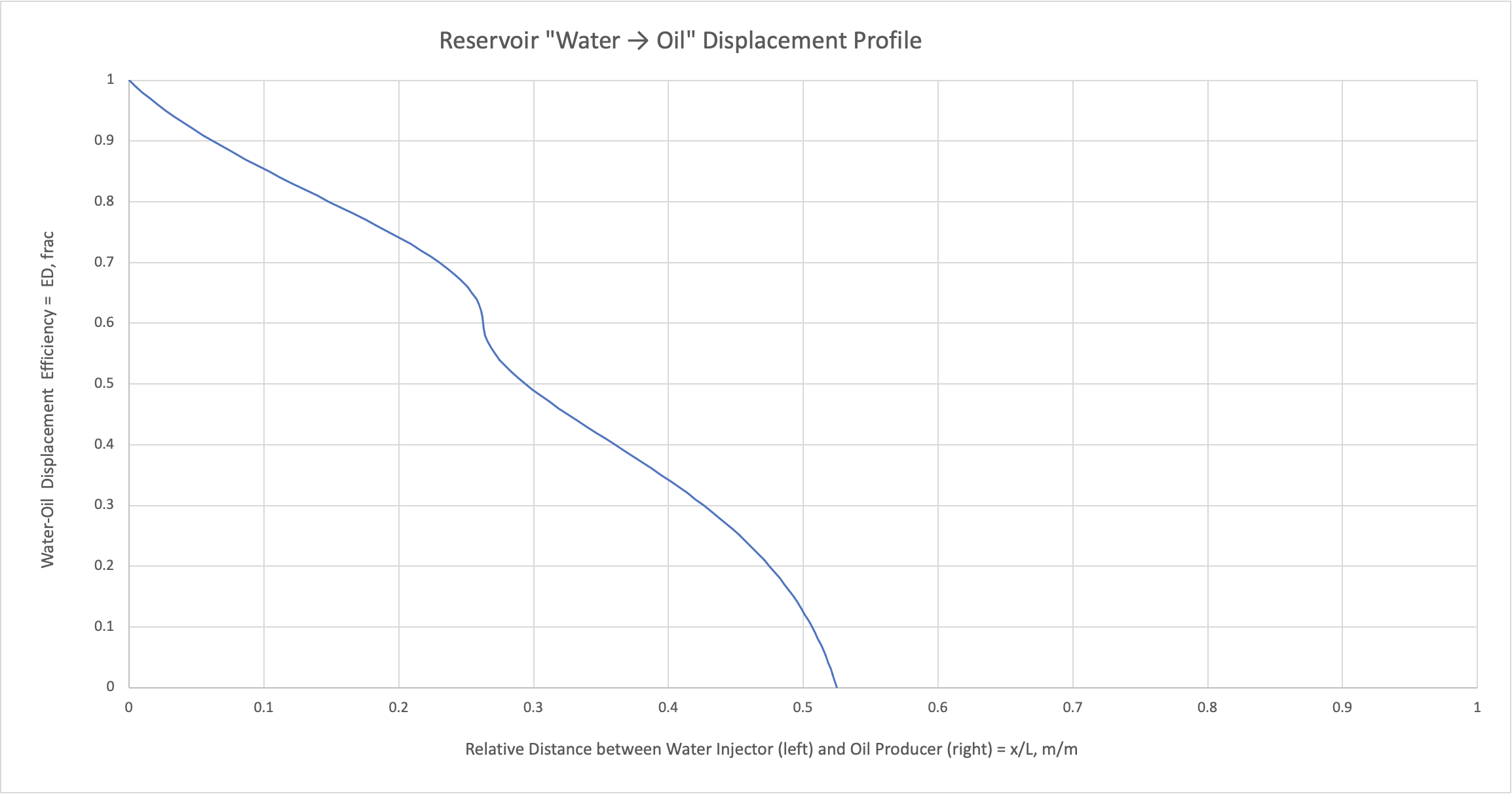 Image Added Image Added
| Fig. 1 – Sample case of Buckley–Leverett reservoir saturation profile capturing the moment,when water front is still on mid-way towards the producing well, sitting at | LaTeX Math Inline |
|---|
| body | x_D = 1 \Leftrightarrow x = L |
|---|
|
. |
|
|
|