...
| field-average formation pressure within the drainage area of a given well: | LaTeX Math Inline |
|---|
| body | p_R = \frac{1}{V_e} \, \int_{V_e} \, p(t, {\bf r}) \, dV |
|---|
|
|
Water and Dead Oil IPR
...
Based on these notions above defintions the general WFP – Well Flow Performance can be wirtten in universal a general form:
| LaTeX Math Block |
|---|
|
p_{wf} = p_R - \frac{q}{J_s} |
...
| for producer |
| for injector |
| LaTeX Math Inline |
|---|
| body | q=q_{\rm liq}=q_o+q_w |
|---|
|
| for oil producer |
| for gas producer or injector |
| for water injector or water-supply producer |
The Productivity Index can be constant or dependent on bottom-hole pressure
.
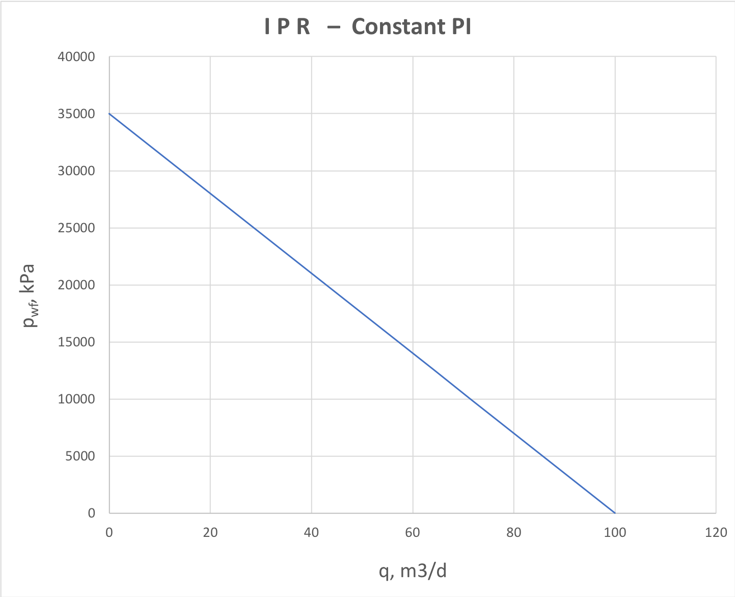
For a single layer formation with low-compressibility fluid (like water or dead oil) the PI does not depend on drawdown (or flowrate)
and
WFP – Well Flow Performance plot is reperented by a straight line (Fig. 1)
...
This is a typical WFP – Well Flow Performance plot for water supply wells, water injectors and dead oil producers above bubble point.
The PI can be estimated using the Darcy equation:
...
for steady-state
SS flow and
for pseudo-steady state
PSS flow.
...
For gas producers, the fluid compressibility is high and formation flow in well vicinity becomes non-linear (deviating from Darcy) fot high flowrates, inflicting the downward trend on WFP – Well Flow Performance plot (Fig. 2).
...
In general case of saturated oil, the PI
features a complex dependance on bottom-hole pressure
( or flowrate
) which can be etstablished based on numerical simulations of multiphase formation flow.
But when field-average formation pressure is above bubble-point
(which means that most parts of the drainage area are saturated oil) the
PI can be farily approximated by some analytical correlations.
Saturated Oil IPR
...
For 2-phase oil-gas formation flow below bubble point
the free gas slippage effects inflict the downward trend on
WFP – Well Flow Performance plot (Fig. 3).
...
Multiphase IPR
...
For 3-phase water-oil-gas flow the IPR analysis is perfomed on oil and watr components (see Fig. 4.1 and Fig. 4.2).
...