Mathematical model of rock shaliness.
The shales contain much higher concentration of radioactive minerals comparing to clean sands and carbonates (see Table 1 below).
This is why the most common way to quantify the shale content is the intensity of the natural gamma-ray (GR) emission.
The fist step is to normalize the actual GR-tool readings GR_{log} to the reference values in clean rocks GR_m and pure shales GR_{sh} which is called Shale Index:
| (1) | I_{GR}(l) = \frac{GR_{log}(l) - GR_m}{GR_{sh} - GR_m} |
where l – along-hole depth.
The model parameters GR_{sh} and GR_m are calibrated for each facies individually.
The shale Index I_{GR} is varying between 0 (for non-shally rocks) and 1 (for pure shales) but the actual shaliness may behave non-linearly between these extremes (especially for shallow, young reservoirs).
This can be calibrated based on the available core data.
The table below summairzes some popular shaliness models:
| # | Equation | Author | Rock Type | Correlation database |
|---|---|---|---|---|
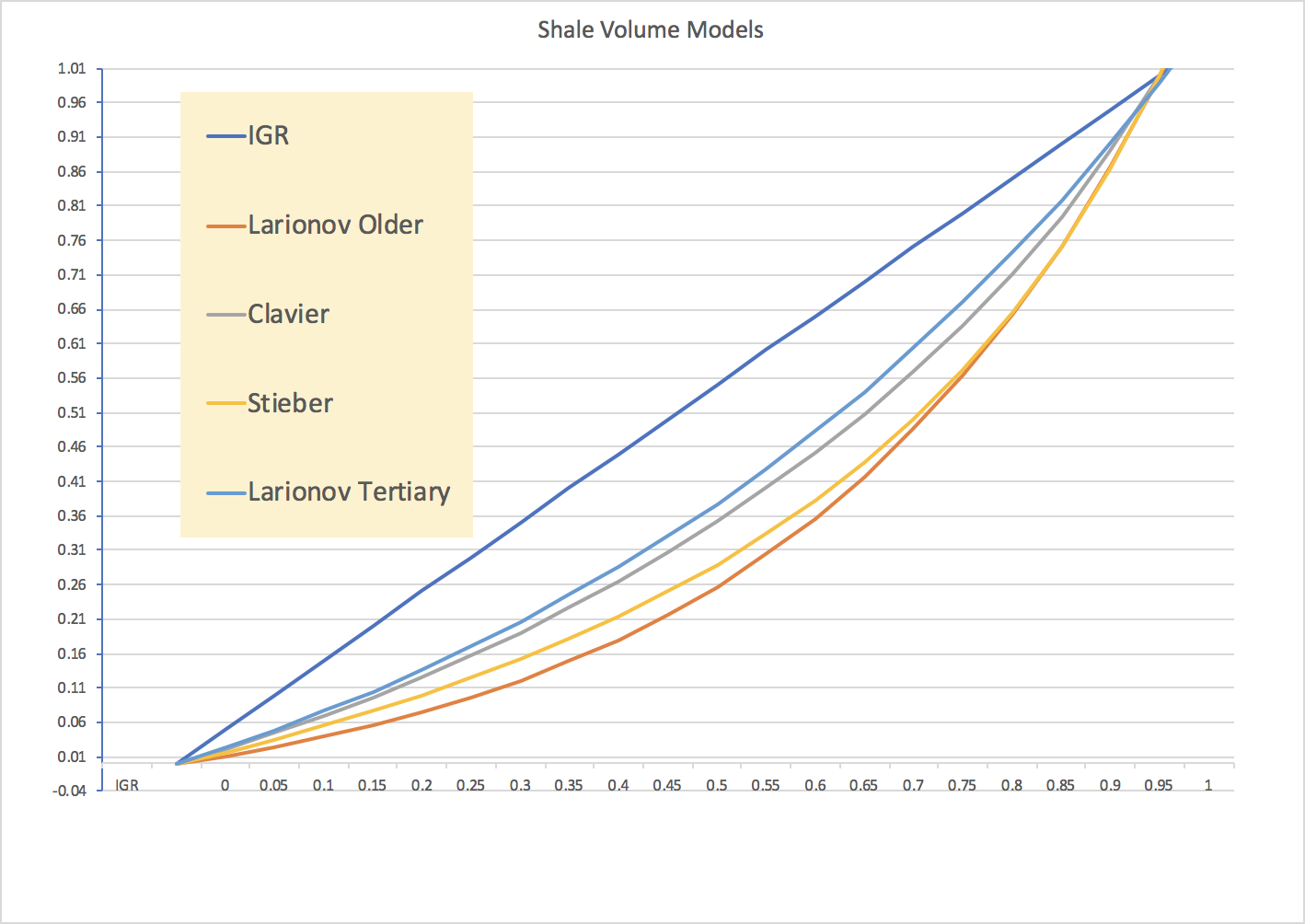
| 1 | V_{sh} = I_{GR} | |||
| 2 | V_{sh} = 0.083 \cdot (2^{3.7 I_{GR}} - 1) | Larionov (1969) | Tertiary Jurassic rocks | West Siberia |
| 3 | V_{sh} = 1.7 - \sqrt{(3.38 - (I_{GR}+0.7)^2)} | Clavier (1971) | ||
| 4 | V_{sh} = \frac{ I_{GR}}{3 - 2 I_{GR}} | Stieber (1970) | ||
| 5 | V_{sh} = 0.33 \cdot (2^{2 I_{GR}} - 1) | Larionov (1969) | Older Rocks | West Siberia |
The graphic image of different shales volume models is brought on Fig. 1.
| Table 1. GR values for popular minerals | ||||
| Rock Type | GR, API | ||
| 1 | Halite (NaCl) | 0 | ||
| 2 | Coal | 0 | ||
| 3 | Limestone | 5 – 10 | ||
| 4 | Sandstone | 10 – 20 | ||
| 5 | Dolomite | 10 – 20 | ||
| 6 | Shale | 80 – 140 | ||
| 7 | Mica | 100 – 170 | ||
| 8 | Silvite (KCl) | 500 | ||
| Fig. 1. Shale Volume Models. | ||||