Fluid flow with fluid pressure $\begin{array}{l}p(t, {\bf r})\end{array}$ linearly changing in time:

$\begin{array}{l}\displaystyle p(t, {\bf r}) = \psi({\bf r}) + A \cdot t, \quad A = \rm const\end{array}$

The fluid temperature $\begin{array}{l}T(t, {\bf r})\end{array}$ is supposed to vary slowly enough to provide quasistatic equilibrium.

The fluid velocity $\begin{array}{l}{\bf u}(t, {\bf r})\end{array}$ may not be stationary.

In the most general case (both reservoir and pipelines) the fluid motion equation is of fluid pressure and pressure gradient:

(1)	$\begin{array}{l}\displaystyle {\bf u}(t, {\bf r})= F({\bf r}, p, \nabla p)\end{array}$

with right side dependent on time through the pressure variation.

In case of the flow with velocity dependent on pressure gradient only $\begin{array}{l}{\bf u} = {\bf u}({\bf r}, \nabla p)\end{array}$ ) the PSS flow velocity will be stationary as the right side of (1) is not dependant on time.

In terms of Well Flow Performance the PSS flow means:

(2)	$\begin{array}{l}\displaystyle q_t(t) = \rm const\end{array}$

(3)	$\begin{array}{l}\displaystyle \Delta p(t) = \| p_e(t) - p_{wf}(t) \| = \Delta p = \rm const\end{array}$

During the PSS regime the formation pressure also declines linearly with time: $\begin{array}{l}p_e(t) \sim t\end{array}$ .

The exact solution of diffusion equation for PSS:

(4)	$\begin{array}{l}\displaystyle p_e(t) = p_i - \frac{q_t}{ V_{\phi} \, c_t} \ t\end{array}$

varying formation pressure at the external reservoir boundary

(5)	$\begin{array}{l}\displaystyle p_{wf}(t) = p_e(t) - J^{-1} q_t\end{array}$

varying bottom-hole pressure

(6)	$\begin{array}{l}\displaystyle J = \frac{q_t}{2 \pi \sigma} \left[ \ln \left ( \frac{r_e}{r_w} \right) +S + 0.75 \right]\end{array}$

constant productivity index

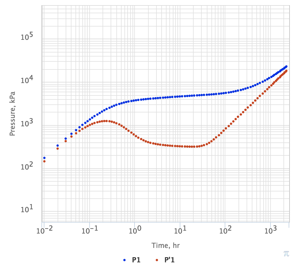
and develops a unit slope on PTA diagnostic plot and Material Balance diagnostic plot:

Fig. 1. PTA Diagnostic Plot for vertical well in single-layer homogeneous reservoir with impermeable circle boundary (PSS).

Pressure is in blue and log-derivative is in red.

Page tree

See Also

Page tree

Pseudo Steady State (PSS) fluid flow

See Also